Calculating Number Needed to Treat/Harm (NNT/H) with Odds Ratio

We learned how to convert the pooled odds ratio from a random-effects model and subsequently calculate the number needed to treat (NNT) or harm (NNH). It’s important to understand that without knowing the event proportions in either the treatment or control groups, we cannot accurately estimate the absolute risk reduction for an individual study or for a meta-analysis. Fascinating indeed! Everyday is a school day! 🙌

.
Image generated via DALL-E

Last week, we have demonstrated how to calculate event proportion of treatment and control group with random effect weights, and use it to eventually calculate NNT. Now, we will learn how to convert odds ratio to NNT.

Objectives:

• Breaking down odds ratio
• Calculating random effect pooled odds ratio
• Converting Odds ratio to Event Proportion
• Calculate NNT
• Lessons Learnt

Breaking down odds ratio

$$\begin{gather} \text{Odds ratio} = \frac{\text{Odds}_t}{\text{Odds}_c} \\ \text{Odds ratio} = \frac{\frac{\text{Event}_t}{n_t-\text{Event}_t}}{\frac{\text{Event}_c}{n_t-\text{Event}_c}} \end{gather}$$

\(\text{Odds}_t\): Odds for treatment group
\(\text{Odds}_c\): Odds for control group
\(\text{Event}_t\): Event count for treatment group (e.g., how many patients are cured after treatment)
\(n_t\): Total patients in treatment group
\(\text{Event}_c\): Event count for control group (e.g., how many patients are cured after placebo)
\(n_c\): Total patients in control group

Let’s look at Effect of Remdesivir vs Standard Care on Clinical Status at 11 Days in Patients With Moderate COVID-19 Spinner C et al JAMA. 2020 Sep 15; 324(11): 1–10..) as an example.

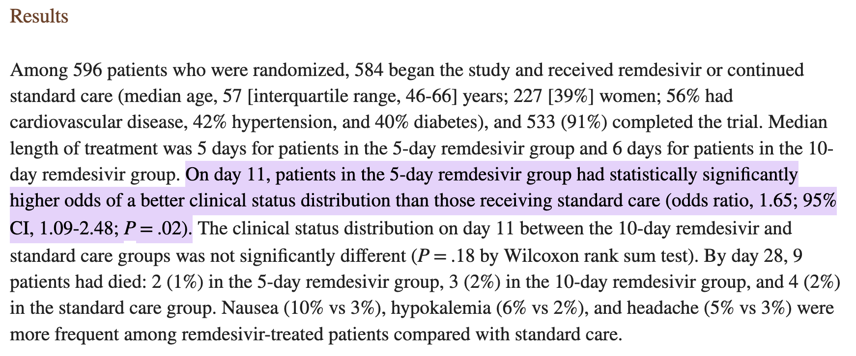
Let’s see if we can get close to that odds ratio using information provided by the manuscript. Let’s see if we can get to OR 1.65. Looking at 5-day remdesivir group, we have \(n_t\) of 191 and standard of care \(n_c\) of 200. Through table 2, we see that 134 \(event_t\) in treatment group had clinical improvement and 121 \(event_c\) in SOC group had clinical improvement.

Given the information above, to calculate OR, it would be: $$\begin{gather} \text{Odds ratio} = \frac{\frac{134}{191-134}}{\frac{121}{200-121}} \\ \text{Odds ratio} = 1.534 \end{gather}$$

Close enough for calculating simple odds ratio. 🤷‍♂️ The study uses proportional odds model, which the supplement did say that there were adjustments for certain variables. Hence, it’s more of an exp(coef) from the proportional odds model than calculation above. But for our demonstration purposes, that is how one calculates odds ratio.

Since we know how odds ratio come about, one could see that we can easily then convert these numbers to event proportions for both treatment and control groups, which in turn we can then calculate absolute risk reduction and eventually NNT! Event proportion on treatment group would be 134/191 = 0.7015707, and event proportion on control group would be 121/200 = 0.605. ARR would be 0.702-0.605=0.097. Hence NNT would be 1/0.097 = 12! Yes, we did it!

What If We Don’t Have The Actual Counts?

If we don’t have the actual counts (in our case we do but since we cannot reconstruct their proportional odds model, we cannot directly calculate odds ratio that is exactly their value), we then at least need a baseline / control event proportion to further estimate treatment event proportion. Without either of these information, I’m afraid we cannot estimate ARR and NNT accurately.

What if we do have control group even porportion, how do we then back-calculate to get the treatment event proportion?

$$\begin{gather} \text{Odds ratio} = \frac{\frac{\text{Prop}_t}{1-\text{Prop}_t}}{\frac{\text{Prop}_c}{1-\text{Prop}_c}} \end{gather}$$ \(\text{Prop}_t\): Event proportion for treatment group (e.g., what percentage of patients are cured after treatment)
\(\text{Prop}_c\): Event proportion for control group (e.g., what percentage patients are cured after placebo)

Let’s take our event proportion for control group is 0.605, and OR of 1.534, let’s back-calculate and see if we can get bacck to 0.702 for event proportion of treatment group.

$$\begin{gather} 1.534 = \frac{\frac{\text{Prop}_t}{1-\text{Prop}_t}}{\frac{0.605}{1-0.605}} \\ 1.534 = \frac{\frac{\text{Prop}_t}{1-\text{Prop}_t}}{1.532} \\ 1.534\cdot1.532 = \frac{\text{Prop}_t}{1-\text{Prop}_t} \\ 2.35 = \frac{\text{Prop}_t}{1-\text{Prop}_t} \\ 2.35\cdot(1-\text{Prop}_t) = \text{Prop}_t \\ 2.35 - 2.35\text{Prop}_t = \text{Prop}_t \\ 2.35 = \text{Prop}_t + 2.35\text{Prop}_t \\ 2.35 = 3.35\text{Prop}_t \\ \text{Prop}_t = \frac{2.35}{3.35} \\ \text{Prop}_t = 0.70149 \\ \end{gather}$$

Et Viola! Very very close to our previous number!

Visualizing p1 (treatment event proportions) vs p0 (control event proportions) That Makes Up OR 1.534

library(tidyverse)

eg <- expand_grid(p0=seq(0,1,0.001),p1=seq(0,1,0.001))

eg |>
  mutate(or = p1/(1-p1)/(p0/(1-p0))) |> 
  filter(or > 1.533, or < 1.535) |>
  ggplot(aes(x=p0,y=p1)) +
  geom_point() +
  geom_smooth() +
  theme_minimal()

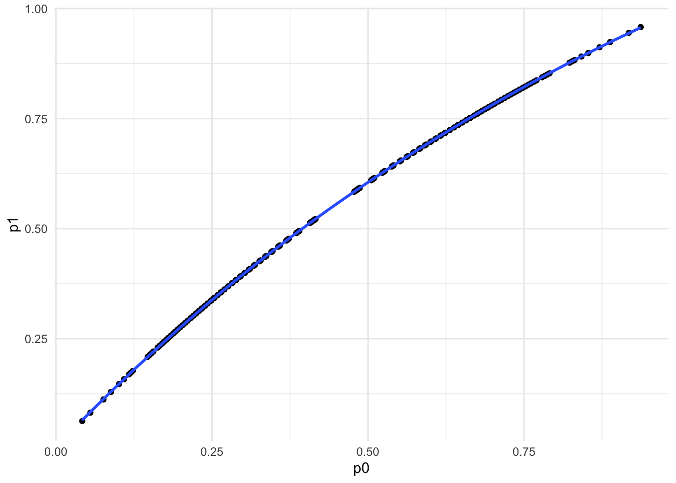
The reason that we cannot calculate ARR and NNT without at least one of the event proportion is because all these combinations shown on the graph can make up OR of 1.534! For example, if treatment event proportion is 0.173, control event proportion should be 0.12 to make or OR of 1.534. Event proportions clearly are not the same as our previous reported numbers clerly have the same OR.

Guess what? If we have different event proportion we may not have the same difference of event proportion (ARR), especially if they don’t follow a straight line. Let’s take a look at random sampling of 20 experiments and see what their ARR and NNT are.

eg |>
  mutate(or = p1/(1-p1)/(p0/(1-p0))) |> 
  filter(or > 1.533, or < 1.535) |>
  mutate(arr = p1-p0,
         nnt = ceiling(1/arr)) |>
  slice_sample(n = 20) |> view()

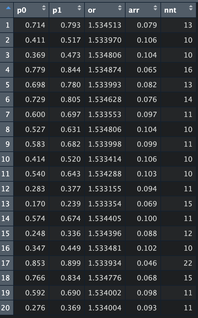
Notice that ARRs are quite different, sure sometimes we may get lucky that the NNT might be close to our calculated NNT, but it would not have come from accurate event proportions.

Calculating Random Effect Pooled Odds Ratio

Let’s take a look at this article Association of Gastric Acid Suppression With Recurrent Clostridium difficile Infection A Systematic Review and Meta-analysis R Tariq JAMA Intern Med. 2017;177(6):784-791

library(meta)

df1 <- tibble(study=c("Abdelfatah 2015","Cadena 2010","Cadle 2007", "Freedberg 2013", "Hebert 2013", "Hikone 2015", "Khanna 2012","Kim 2010", "Kim 2012", "Linsky 2010", "McDonald 2015","Moshkowitz 2007", "Rodriguez-Pardo 2013","Samie 2013","Tal  2002","Weiss 2015"),event.c=c(78,0,7,74,120,2,79,10,7,118,61,9,14,1,20,33),n.c=c(1038,1,43,343,578,16,245,69,18,639,235,38,107,29,47,219))

df2 <- tibble(study=c("Abdelfatah 2015","Cadena 2010","Cadle 2007", "Freedberg 2013", "Hebert 2013", "Hikone 2015", "Khanna 2012","Kim 2010", "Kim 2012", "Linsky 2010", "McDonald 2015","Moshkowitz 2007", "Rodriguez-Pardo 2013","Samie 2013","Tal  2002","Weiss 2015"),event.t=c(131,38,40,93,78,12,37,17,14,133,132,5,48,19,23,72),n.t=c(981,128,97,551,251,60,140,56,24,527,411,13,208,75,34,482))

df <- df1 |>
  full_join(df2, by = "study") 

def <- metabin(event.c = event.c,n.c = n.c, event.e = event.t, n.e = n.t, studlab = study,data = df,sm="OR",level = 0.95,comb.fixed=T,comb.random=T,hakn = F, method.tau = "REML",overall = T)

summary(def)
forest(def)

Summary of the meta-analysis:

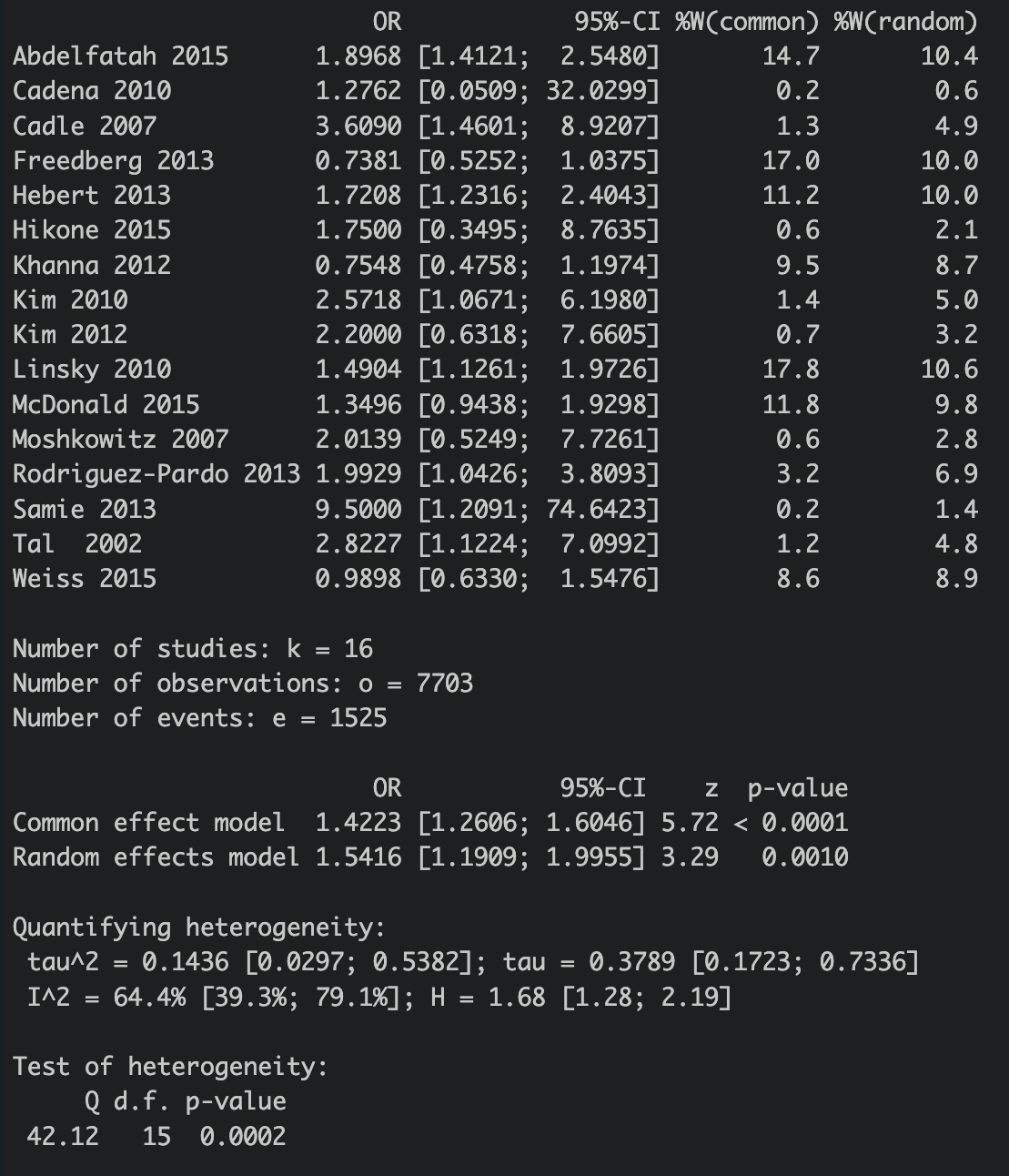
Forest plot:

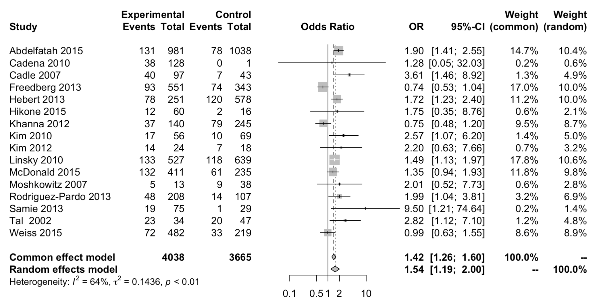
Alright, now that I had {meta} do the magic random effect for me, how on earth do I then use this aggregated OR to further calculate ARR and then NNT? One may say, well, we have all these numbers, can’t we just total them up? We can’t, but let’s try and see how wrong our answer is.

So, if we were to think event proportion for treatment group is \(\frac{\sum{event_t}}{\sum{n_t}}\) = \(\frac{892}{4038}\) = 0.221. Event proportion for the control group is \(\frac{\sum{event_c}}{\sum{n_c}}\) = \(\frac{633}{3665}\) = 0.173. ❌

Let’s take a look at our numbers that are influenced by the random effect weights.

weights <- def$w.random / sum(def$w.random)

df_new <- df |>
  mutate(weights = weights,
         log_c = log(event.c/(n.c-event.c))*weights,
         log_c = case_when(
           event.c == 0 ~ log(0.5/(n.c-0.5))*weights,
           TRUE ~ log_c),
         log_t = log(event.t/(n.t-event.t))*weights,
         log_t = case_when(
           event.t == 0 ~ log(0.5/(n.t-0.5))*weights,
           TRUE ~ log_t),
         log_c_prop = log(event.c/n.c)*weights,
         log_c_prop = case_when(
           event.c == 0 ~ log(0.5/n.c)*weights,
           TRUE ~ log_c_prop
         ))

# average odds  on treatment
odds_t <- exp(sum(df_new$log_t) / sum(weights))

# average odds  of control
odds_c <- exp(sum(df_new$log_c) / sum(weights))


# odds ratio
odds <- odds_t / odds_c

prop_c <- odds_c / (1+odds_c)
prop_t <- odds_t / (1+odds_t)


## NNT
arr <- prop_t - prop_c         

var_arr <- prop_t * (1-prop_t) / sum(df_new$n.t) + prop_c * (1-prop_c) / sum(df_new$n.c)
nnt_l3 <- ceiling(1/abs(arr - 1.96*sqrt(var_arr)))

# NNT upper
nnt_u3 <- ceiling(1/abs(arr + 1.96*sqrt(var_arr)))

nnt_ci_3 <- paste0(ceiling(1/arr)," [95%CI ",nnt_u3, "-",nnt_l3,"]")

✅ Our event proportion for treatment group is 0.2641518 and our event proportion for control group is 0.1899116. Quite different isn’t it? Our calculated OR is 1.5312512, quite similar to the forest plot, hurray! If you are interested in how to use those weights, please visit my previous blog. I basically replaced proportion equation to odds equation.

Converting Odds ratio to Event Proportion

How do we then back-calculate the event proportion using our odds? Let’s just take a look at odds for treatment. Our aggregated odds for treatment is 0.358976

$$\begin{gather} \text{Odds}_t = \frac{\text{Prop}_t}{1-\text{Prop}_t} \\ \text{Odds}_t \cdot (1-\text{Prop}_t) = \text{Prop}_t \\ 0.358976 \cdot (1-\text{Prop}_t) = \text{Prop}_t \\ 0.358976 - 0.358976(\text{Prop}_t) = \text{Prop}_t \\ 0.358976 = \text{Prop}_t + 0.358976(\text{Prop}_t) \\ 0.358976 = 1.358976(\text{Prop}_t) \\ \text{Prop}_t = \frac{0.358976}{1.358976} \\ \text{Prop}_t = 0.2641518 \end{gather}$$

Not too shabby! Exact number, sweet! There is also another simple equation where \(prop_t = \frac{\text{odds}_t}{1+\text{odds}_t}\). You can do the same for \(prop_c\) as well which I will not repeat.

Calculate NNT

This part should be simple, since we have \(prop_t\) and \(prop_c\). Let’s calculate ARR which is \(prop_t - prop_c\) = 0.0742403. NNT is \(\frac{1}{ARR}\) = 14 [95%CI 11-18].

So, with this study, it’s not appropriate to call it Number Needed To Treat since what we’re measuring is the harm 👿 of treatment compared to no treatment, we call this Number Needed To Treat and Harm or Number Needed to Harm (NNTM or NNH). Essentially, what we’re saying, given this aggregated odds ratio with random effect, is for every 14 patients we treat with PPI, we may expect 1 case of Clostridiodes difficile colitis, when compared to those who’s not on PPI.

Lessons Learnt

• Random effect odds ratio calculation is quite similar to previous, please let me know if there is mistake or if you’d like me to elaborate more here on this blog
• Learnt to use fig.show='hide'
• Learnt to use group in {meta}, though not shown here. This would be helpful when the random effect is pooled from both adjusted and unadjusted studies where you can see the different estimates prior to total pooled estimates.

If you like this article:

• please feel free to send me a comment or visit my other blogs
• please feel free to follow me on twitter, GitHub or Mastodon
• if you would like collaborate please feel free to contact me