S.P.I.C.E of Causal Inference

The SUTVA, Positivity, Identifiability, Consistency, Exchangeability of Causal Inference, the essential ingredients that helps us bring out the true flavor of the causal model. Here is my understanding of each assumptions (main course) with examples (side dish) and accompanied by simulation (paired with beverages). Bon Appétit!

Since the multiple readings of The Book of Why which piqued my interest in causal inference, and then further layperson’s language and knowledge provided by Causal Inference and Discovery in Python, I am very motivated in learning more about causal inference. Judea Pearl is right, our brain is wired to think causally.

Almost all research questions I have encountered since medical school we’re always interested in causality. Even when we’re actually using descriptive statistics to describe something, we never failed to use causal language to “conclude” or “infer” our findings. E.g. We see a positive asociation between X and Y, hence we think X may be causing Y, and then buffer it with language of uncertainty e.g. a larger, randomized experiment should be conducted to further answer the question of interest. 🤷‍♂️

And of course the phrase Correlation does not imply causation has been ingrained in our heads (of course for a good heuristic reason), but also constrained our thinking that causation cannot be identified with observational studies. Please do not get me wong, 🤣, the extreme end of the other side, e.g., we can identify everything with causal inference, is also a danger zone, just like the retropharyngeal space. Nonetheless, if one were to use causal inference as a tool, one MUST understand the fundamentals of its assumptions, just like any other statistical tools. With that in mind, this is my watered-down version of CI assumption notes, mainly for me to review in the future whenever I forget what each of these terminology means.

SPICE

FYI, I will continue to modify, edit, and revise anything wrong in order for me to continue to learn and grow in this wonderful CI world. From my learning, I figured a mnemonic that would work for me is SPICE! No, I’m not talking about amp-c, that mneumonic no longer follows the recent guideline anyway. But I meant SUTVA, Positivity, Identifiability, Consistency, Exchangeability.

Disclaimer

From the languages and terminology that I used or perhaps misused, it is clear that I am a beginner in this topic. If you noticed any inconsistency, insufficiency, non-identifiability, non-transportability of the information I have presented. Please guide me to the truth. I am happy to revisit the topic, revise, and learn! As usual, this is not a medical or statistical advice, please consult your physician and statistician.

Objectives

• What Does Spice Stand For?
  • Disclaimer
• SUTVA
• Positivity Assumption
• Identifiability
• Consistency
• Exchangeability
• Cheat Sheet
• Lessons Learnt

SUTVA

The Stable Unit Treatment Value Assumption (SUTVA) is a fundamental principle in causal inference, particularly in the context of randomized experiments and observational studies. It asserts two main conditions for the analysis of causal effects.

First, the treatment assigned to one unit does not affect the outcome of another unit, meaning there are no interference or spillover effects between units. This aspect is often summarized as “no interference.”. This is the one we will simulate below.

Second, the potential outcomes for any unit are the same under the same treatment level, regardless of the mechanism or path through which the unit received the treatment. This means that the treatment effect is consistent across different units and there’s no variation in treatment effects based on how the treatment is administered. This is the C in SPICE.

SUTVA 1

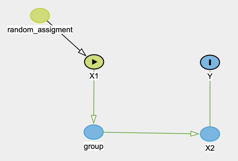
The DAG above depicts an unblinded random assignment (50%) of treatment to X1. However, X1 resides in groups. And for some reason, if each group contains more than 50% treatment, then the treatment is no longer 50% but 80%. The outcome then will be influenced by the new treatment assignment X2 instead, which is not observed or measured in reality. And we will erroneously estimate the treatment effect of X1 instead. Several examples would be exercise vs no exercise or coaching vs no-coaching.

In the exercise example, imagine exercises and no-exercises were assigned to certain people through the school as treatment and control group, since this is unblinded, the exercise group may share that they’re going to gym more often, influencing their classmates to join them as well. When all school mates were assessed for certain outcome, say, happiness/wellness score, we estimated the treatment effect with the orginal treatment assignment group, which can also be known as total effect. However, remember only if the class contains more than 30% of exercise-prescribed students will it have mediating effect to the rest of the class, otherwise it won’t. Now this is a violation of SUTVA #1. We can apply this to coaching vs no-coaching as well. Imagine if more than 30% of students in the classed were coached and produced a more positive perspective of life and future, which then spreads throughout the class.

library(tidyverse)

set.seed(1)
n <- 1000
x1 <- rbinom(n, 1, 0.5)
group <- replicate(n, expr = sample(1:50, 1))


df <- tibble(x1,group) |>
  group_by(group) |>
  mutate(x1_mean = mean(x1)) |> 
  mutate(x2 = map2_int(.x=x1_mean, .y=x1, .f=~ if (.x > 0.5 & .y != 1) { sample(0:1, 1, prob = c(0.2,0.8), replace = F) } else if (.y == 1) { .y } else { sample(0:1, 1, prob = c(1-.y,.y), replace = F) } )) |>
  ungroup(group) |>
  mutate(y = map_dbl(.x=x2, .f=~rbinom(n=1, size=1, plogis(2*.x))))

model_wrong <- glm(y~x1,df,family="binomial")

summary(model_wrong)

## 
## Call:
## glm(formula = y ~ x1, family = "binomial", data = df)
## 
## Deviance Residuals: 
##     Min       1Q   Median       3Q      Max  
## -1.9845  -1.3752   0.5483   0.9917   0.9917  
## 
## Coefficients:
##             Estimate Std. Error z value Pr(>|z|)    
## (Intercept)  0.45378    0.08997   5.044 4.57e-07 ***
## x1           1.36497    0.15950   8.558  < 2e-16 ***
## ---
## Signif. codes:  0 '***' 0.001 '**' 0.01 '*' 0.05 '.' 0.1 ' ' 1
## 
## (Dispersion parameter for binomial family taken to be 1)
## 
##     Null deviance: 1164.5  on 999  degrees of freedom
## Residual deviance: 1082.8  on 998  degrees of freedom
## AIC: 1086.8
## 
## Number of Fisher Scoring iterations: 4

Wow, OK, let’s break down the codes in a bit.

1. We simulated x1 with a random assignment with probability of 50% of control (0) vs treatment (1).
2. We then randomly sample from 1 to 50, nth time, to allocate groups for each observation / subject and save it in group.
3. Create a dataframe with both xq and group variable.
4. Group our groups and then calculate mean of x1 and save it under x1_mean.
5. x2 assignment:
   • if x1_mean is > 50% and x1 is not a 1, then randomly sample with probability of 20% for 0 and 80% for 1.
   • if x1 is already 1, then x2 should also be 1
   • everything else, randomly sample 50-50
6. Assign y with a random variable from binomial distribution of inverse logit of 2*x2. Our coefficient of interest should be 2.
7. Regress y with x1 to false estimate our coefficient.

Interpretation:

As we can see, our wrong model estimated that x1 has positive effect on y, when in fact it shouldn’t have any direct effect on y. We know this because we generated the data that way mutate(y = map_dbl(.x=x2, .f=~rbinom(n=1, size=1, plogis(2*.x)))). Looking at the last line of data generating process in the code above. Otherwise, see below for y regressing on x1 and x2:

model_right <- glm(y~x1+x2,df,family="binomial")

summary(model_right)

## 
## Call:
## glm(formula = y ~ x1 + x2, family = "binomial", data = df)
## 
## Deviance Residuals: 
##     Min       1Q   Median       3Q      Max  
## -2.0963  -1.2018   0.5483   0.5483   1.1532  
## 
## Coefficients:
##             Estimate Std. Error z value Pr(>|z|)    
## (Intercept)  0.05716    0.10197   0.561    0.575    
## x1          -0.26069    0.30388  -0.858    0.391    
## x2           2.02228    0.29222   6.920 4.51e-12 ***
## ---
## Signif. codes:  0 '***' 0.001 '**' 0.01 '*' 0.05 '.' 0.1 ' ' 1
## 
## (Dispersion parameter for binomial family taken to be 1)
## 
##     Null deviance: 1164.5  on 999  degrees of freedom
## Residual deviance: 1015.6  on 997  degrees of freedom
## AIC: 1021.6
## 
## Number of Fisher Scoring iterations: 4

Remember that x2 and group technically were not measured or observed, hypothetically. The violation of SUTVA here is because the treatment unit is not stable, it actually may lead to control group “getting treatment”, here could be exercise, when proportion of treatment exceeds a certain hypothetical threshold, it changes the initial randomization of treatment.

Positivity

The positivity assumption states that there is a nonzero (ie, positive) probability of receiving every level of exposure for every combination of values of exposure and confounders that occur among individuals in the population - Cole SR Epidemiology 20(1):p 3-5, January 2009.

In short, \(P(Treatment=treatment|Confounders=confounders) > 0\). Which means after adjustment, we should observe all treatments (control vs treatment) in all strata. Below is an example of violation of non-zero probability

# Violate Positivity by ensuring some levels of the confounder never receive treatment
set.seed(1)
n <- 1000
z <- replicate(n = n, sample(0:4,1,replace=T))
x <- ifelse(z > 0, 1, 0)
y <- 0.5*x + 0.6*z + rnorm(n)

summary(lm(y ~ x + z, df))

## 
## Call:
## lm(formula = y ~ x + z, data = df)
## 
## Residuals:
##     Min      1Q  Median      3Q     Max 
## -0.7524 -0.7198  0.2695  0.2766  0.2802 
## 
## Coefficients:
##              Estimate Std. Error t value Pr(>|t|)    
## (Intercept)  0.752381   0.030636  24.559   <2e-16 ***
## x           -0.036106   0.049585  -0.728    0.467    
## z            0.003557   0.014024   0.254    0.800    
## ---
## Signif. codes:  0 '***' 0.001 '**' 0.01 '*' 0.05 '.' 0.1 ' ' 1
## 
## Residual standard error: 0.444 on 997 degrees of freedom
## Multiple R-squared:  0.0006825,	Adjusted R-squared:  -0.001322 
## F-statistic: 0.3404 on 2 and 997 DF,  p-value: 0.7115

model <- glm(x ~ z, df, family = "binomial") 

## Warning: glm.fit: algorithm did not converge

## Warning: glm.fit: fitted probabilities numerically 0 or 1 occurred

Noticed that glm did not like the way we regress x with z, giving warning that algorithm did not converge? That’s a hint of posivitivity violation. Also, notice that the estimates are all wrong!?

Imagine you’re going to the dentist and they score periodontal chart to document your gum health. Typically score the health of your gums from 0–4, with 0 representing health and 4 representing advanced disease. And we have some kind of tooth paste product x that possibly could increase ⬆️ some sort of arbitrary holistic dental health y score, and the higher ⬆️ periodontal score you had z, the better response y you get. Let’s say for people who don’t have teeth, their periodontal score would be 0 (I believe technically they won’t do one if there is no teeth, so this is all just for example sake, not reality), and they would also won’t be using any tooth paste product either. Which is going to be a problem because regardless of how much data we have, we cannot calculate the propensity score of treatment given the confounder. We’ll also be assuming that people with peri score of at least 1 or higher will only seek out this product advertise online.

Let’s break it down how we simulated this in the extreme.

1. Simulate z as 0 to 4 uniformly, n times.
2. Assign x as 1 (use this special product) if peri chart score is 1 or higher, otherwise if z is 0 (people who don’t have teeth) then x will be 0.
3. Generate y, our holistic arbitrary dental health score based on 0.5*.x + 0.6*.y + rnorm(n)

Let’s visualize it

Modelling P(X=x|Z=z)

tibble(z=seq(0,4,0.01), prob=predict(model, newdata = tibble(z=seq(0,4,0.01)), type = "response")) |>
  ggplot(aes(x=z,prob)) +
  geom_point()

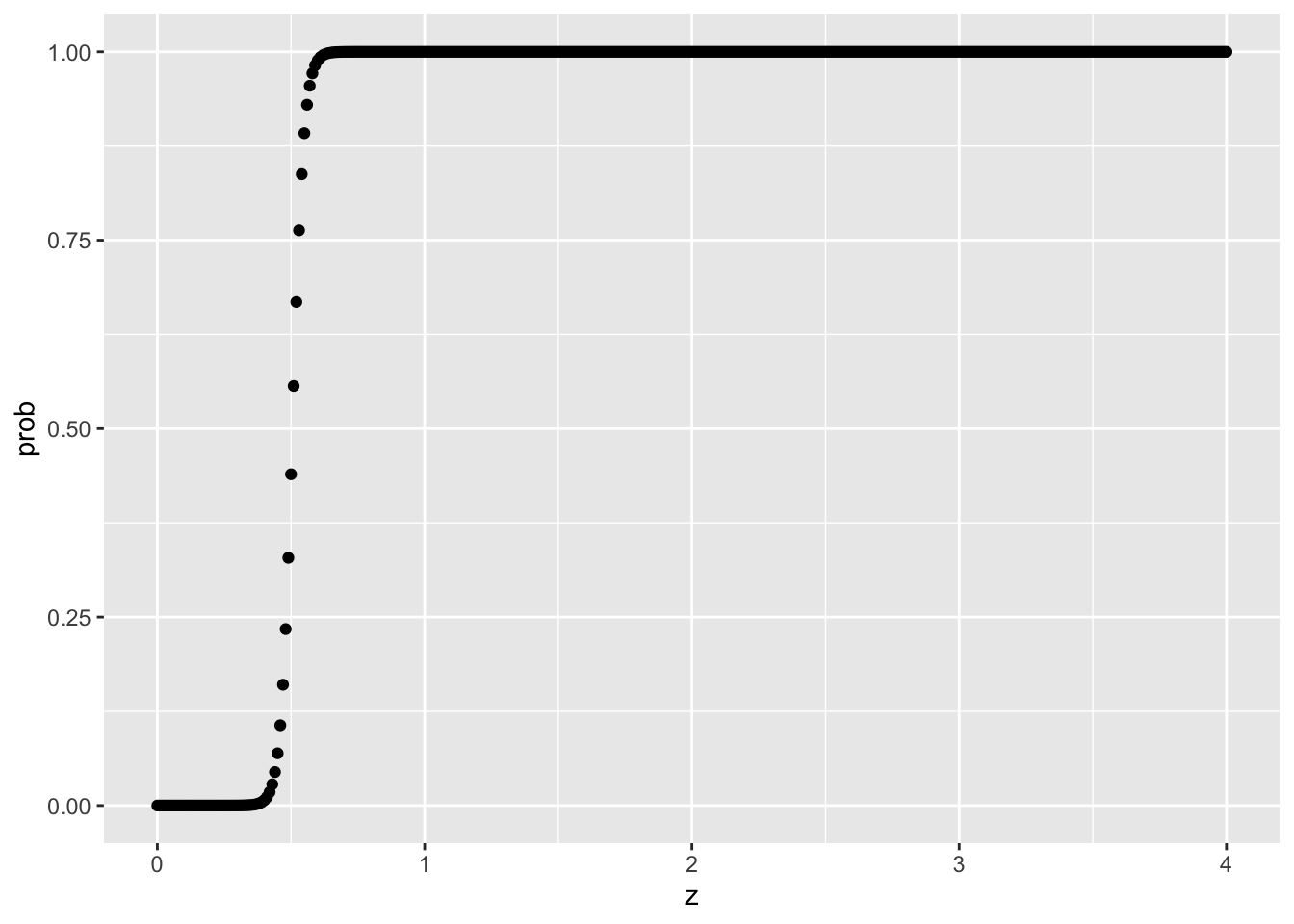
With the above logistic function, notice how z of 0 will have 0% probability of receiving treatment, and z >= 1 will have 0% probability of NOT having treatment either. That’s a no-no!

tibble(x,y,z) |>
  ggplot(aes(x=z,y=y,color=as.factor(x))) +
  geom_point()

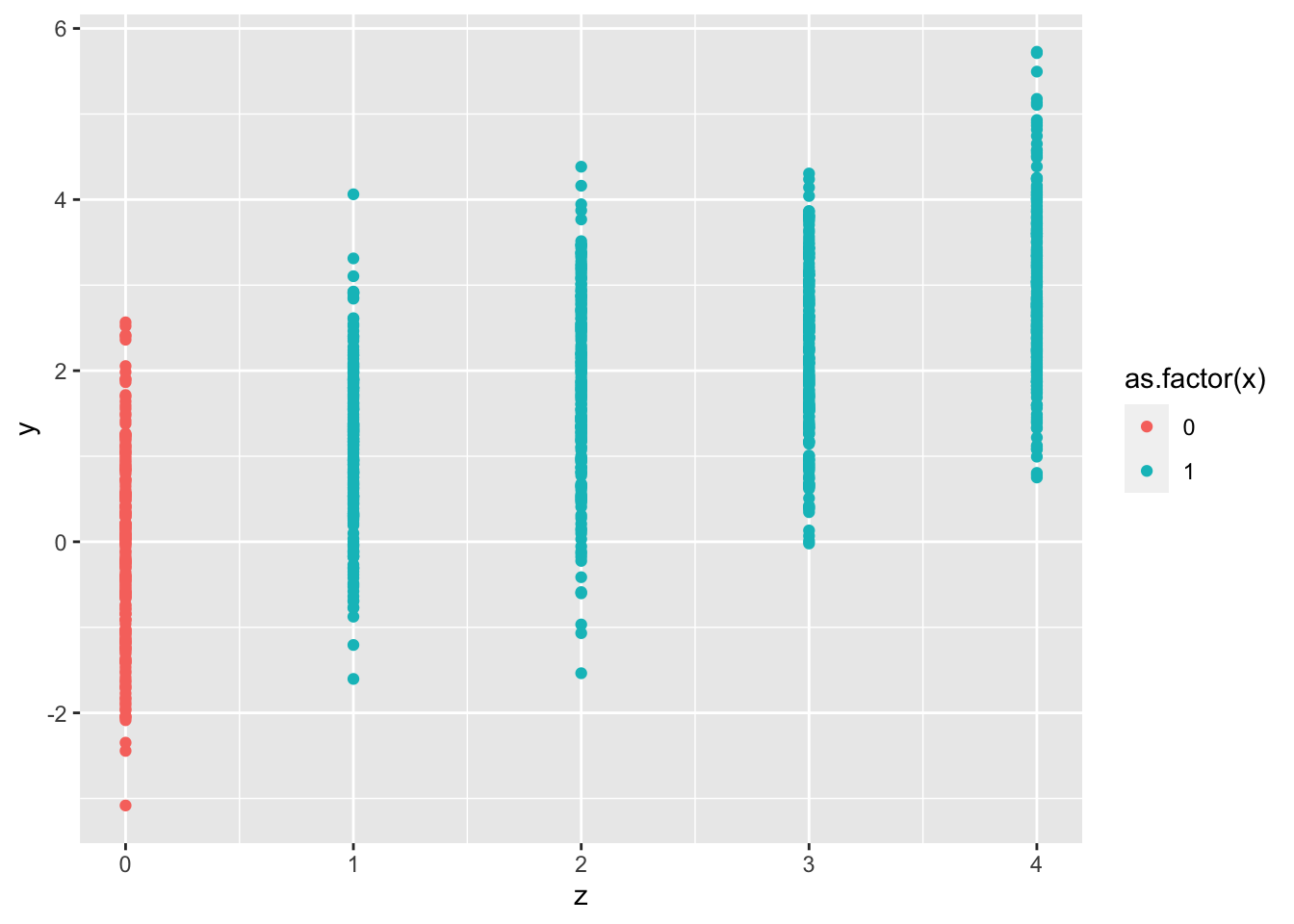
Same here, looking at the colors, we clearly see that all red is in Z=0, and all blue/turqoise are in 1,2,3,4. Positivity assumption violation to the extreme!

Observe that we’ve used so many different characters to represent treatment/exposure, outcome, and confounders. This is something I do find frustrating and confusing. To be clear, in this positivity section, Y is always the outcome, X or T is always the eXposure/Treatment, and W or Z is always the Confounders.

Identifiability

Identifiability refers to the possibility of estimating causal effects from observational data based on specified assumptions, such as the absence of unmeasured confounders and the structure of the causal model. It’s crucial for ensuring that the causal relationships inferred from the data are valid and not confounded by external variables.

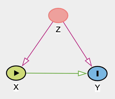
For example, with this DAG below, due to the unobserved or unmeasured nature of confounder Z, we cannot identify causal relationship between X and Y.

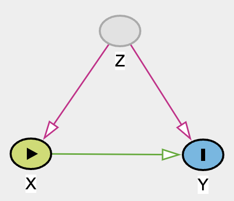
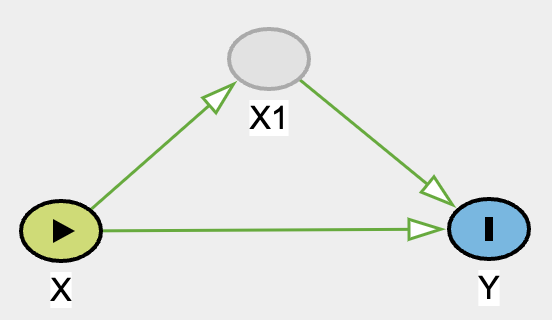
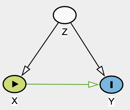
Hence, the violation of identifiability assumption. Regardless of how fancy a method we use for complex data X and Y, we will not be able to draw any useful conclusion of effect X on Y. Unless of course if one can find an instrumental variable IV, magic can occur! See DAG below.

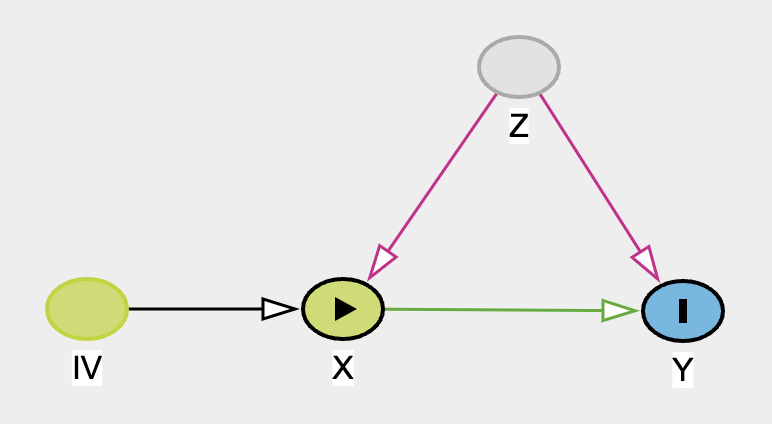
We can estimate the direct effect of X to Y but calculating the total effect and then with some arithmatics, we can identify the direct effect. See here for more total effect = direct effect + indirect effect explaination.

Of course IV is far and few between. It’s more like IV mining! You’ll never know when you can find it. If you did, it’s precious!

Consistency (aka SUTVA 2)

The second assumption of SUTVA, the potential outcomes for any unit are the same under the same treatment level, regardless of the mechanism or path through which the unit received the treatment. This means that the treatment effect is consistent across different units and there’s no variation in treatment effects based on how the treatment is administered.

For example, imagine there is a study that assesses the efficacy of a medication that requires 2 tablets/capsules in order to be the correct dosage for therapeutic effect, but there are some people who took 1 tablet instead of 2. When 1 unit is taken, it may not be as effective. Below we will simulate such scenario.

# no hidden variations of  treatment (consistency)
set.seed(1)
n <- 1000
x <- rbinom(n, 1, 0.5)
x1 <- map_dbl(.x = x, .f = ~ ifelse(.x == 1, sample(c(0, 1), 1, c(0.3,0.7), replace = T), .x)) 
y <- rbinom(n, 1, plogis(-2 + 0.5*x1))

summary(glm(y~x,family="binomial"))

## 
## Call:
## glm(formula = y ~ x, family = "binomial")
## 
## Deviance Residuals: 
##     Min       1Q   Median       3Q      Max  
## -0.5787  -0.5787  -0.5419  -0.5419   1.9956  
## 
## Coefficients:
##             Estimate Std. Error z value Pr(>|z|)    
## (Intercept)  -1.8443     0.1277 -14.441   <2e-16 ***
## x             0.1421     0.1797   0.791    0.429    
## ---
## Signif. codes:  0 '***' 0.001 '**' 0.01 '*' 0.05 '.' 0.1 ' ' 1
## 
## (Dispersion parameter for binomial family taken to be 1)
## 
##     Null deviance: 827.87  on 999  degrees of freedom
## Residual deviance: 827.25  on 998  degrees of freedom
## AIC: 831.25
## 
## Number of Fisher Scoring iterations: 4

OK, let’s break down the code:

1. x: We randomly assign treatment and control group
2. x1: If value is 1, then randomly sample 0 (probability of 30%) and 1 (probability of 70%), otherwise return 0.
   • The reason for this is to emulate the inconsistency of treatment. Imagine 30% of the treatment group took single tablet (inappropriately low dose) which shouldn’t give a therapeutic effect
   • Of course, this is an unobserved variable
3. y: This is the outcome. And the true effect should be 0.5.

However, when we regress y with x, we incorrectly estimated the treatment effect of the medication since 30% of treatment group technically didn’t get a therapeutic dose. This is a hidden variation of treatment, violation of consistency assumption.

Exchangeability

The exchangeability (or ‘no confounding’) assumption requires that individuals who were exposed and unexposed have the same potential outcomes on average. This allows the observed outcomes in an unexposed group to be used as a proxy for the counterfactual (unobservable) outcomes in an exposed group. RCTs strive to achieve exchangeability by randomly assigning the exposure, while observational studies often rely on achieving conditional exchangeability (or ‘no unmeasured confounding’), which means that exchangeability holds after conditioning on some set of variables. - Causal inference and effect estimation using observational data

For further readings on other discussions/videos I found helpful:

1. Difference between exchangeability and independence in causal inference.
2. Ignorability/exchangeability.

Essentially, the reason that RCT has ignorability is because the outcome is independent of treatment (notation: \(\newcommand{\indep}{\perp \!\!\! \perp} \text{Y} \indep T\)), which also means that we can estimate treatment effect through association of Y and T. If independence can be achieved via closing the backdoor (adjusting for a vector of ALL confounders) (notation: \(\newcommand{\indep}{\perp \!\!\! \perp} \text{Y} \indep \text{T} | \text{X}\)), then same as RCT, we can estimate treatment effect through association of Y and T given X. This concept is more intuitively known as ignorability. But because we can ignore them, we can then have the ability to “exchange” them. Let’s visualize.

Visualizing RCT Exchangeability Table

set.seed(1)
n <- 1000
x <- rbinom(n,1,0.5)
y <- rbinom(n,1,plogis(0.33*x))

df <- tibble(x,y) |>
  mutate(y1 = case_when(
    x == 1 ~ y,
    TRUE ~ NA_integer_
  ),
  y0 = case_when(
    x == 0 ~ y,
    TRUE ~ NA_integer_
  ))

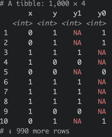
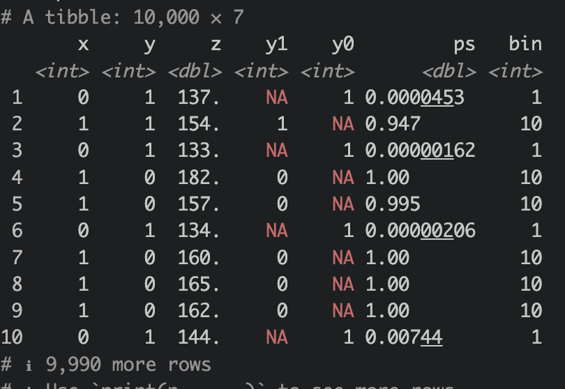
What we have done above is we have simulated a causal relationship of X on Y. Assuming X as treatment (0=control,1=treatment), Y is some sort of favorable outcome (0=no good outcome,1=good outcome). Notice that we use the notation y1 an y0. The notation indicates what the outcome looks like under treatment assignment (e.g., y0 is the outcome when x is 0, y1 is the outcome when x is 1). We sometimes see these nototations (e.g. \(\text{Y}_{(1)}\), or \(\text{Y}^{(1)}\) for observed outcome given treatment=1)

Notice that there are NAs? Of course, we cannot observe these outcomes since the subjects were not given the opposite treatment. However, given ignorability and exchangeability, if treatment were to be swapped, it would be the same as expected outcome of the treatment group like so:

df |>
  mutate(y1 = case_when(
    is.na(y1) ~ mean(y1, na.rm = T),
    T ~ y1
  ),
  y0 = case_when(
    is.na(y0) ~ mean(y0, na.rm = T),
    T ~ y0
  )) 

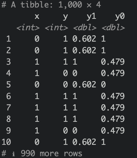
Because this is an RCT, meaning treatment assignment were randomized, assuming blinded as well or at least outcome is not affected by treatment observation, then the average treatment effect is essentially mean(y1) - mean(y0).

Now what about observational study?

set.seed(1)
n <- 10000
z <- rnorm(n, 150,20)
x <- rbinom(n,1,plogis(-120+0.8*z))
# x |> mean()
y <- rbinom(n,1,plogis(120+5*x+-0.8*z))
# y |> mean()

OK, what have we done here? We simulated data where Z influences both X and Y. Let’s give an example of say, we use some kind of fixed dose herbal supplement and we want to observe if the herbal supplement will affect outcome (e.g., happiness, if yes then return a 1 if no then 0). And Z is a blood pressure baseline. For some irrational reason, higher blood pressure increases the probability of taking the herbal supplement, and higher blood pressure decreases happiness score. Here, we simulated that the herbal supplement will have an effect to happiness score. Disclaimer: this is all hypothetical, unrealistic & exaggerated examples are given in order for me to make sense of the DAG. Let’s estimate this incorrectly first.

Wrong estimation ❌

model <- glm(y~x,family=binomial())
summary(model)

## 
## Call:
## glm(formula = y ~ x, family = binomial())
## 
## Deviance Residuals: 
##     Min       1Q   Median       3Q      Max  
## -2.4044  -0.7481   0.3381   0.3381   1.6794  
## 
## Coefficients:
##             Estimate Std. Error z value Pr(>|z|)    
## (Intercept)  2.83342    0.06138   46.16   <2e-16 ***
## x           -3.96386    0.06975  -56.83   <2e-16 ***
## ---
## Signif. codes:  0 '***' 0.001 '**' 0.01 '*' 0.05 '.' 0.1 ' ' 1
## 
## (Dispersion parameter for binomial family taken to be 1)
## 
##     Null deviance: 13473.1  on 9999  degrees of freedom
## Residual deviance:  7662.4  on 9998  degrees of freedom
## AIC: 7666.4
## 
## Number of Fisher Scoring iterations: 5

Here, we wrongly estimated effect of X on Y. Observe that we had simulated a positive effect and yet our wrong model estimated it negatively. Let’s look at ATE.

predict(model,newdata=tibble(x=1),type="response")-predict(model,newdata=tibble(x=0),type="response")

##          1 
## -0.7003753

wrong, wrong, and wong🤣! ❌ But how on earth are we going to deconfounder this and get the right estimates? Enter propensity score stratification (PSS)! Well, there are a lot of other methods, here we’ll be using PSS because it’s more intuitive for this setting. But before we do that, let’s estimate it with our good old logistic regression friend with Z included in our adjustment and estimate our ATE through G-estimation.

Right Model ✅

model <- glm(y~x+z,family=binomial())
summary(model)

## 
## Call:
## glm(formula = y ~ x + z, family = binomial())
## 
## Deviance Residuals: 
##     Min       1Q   Median       3Q      Max  
## -3.3732  -0.0039   0.0000   0.0587   3.0390  
## 
## Coefficients:
##              Estimate Std. Error z value Pr(>|z|)    
## (Intercept) 119.68424    3.85242   31.07   <2e-16 ***
## x             5.13220    0.22341   22.97   <2e-16 ***
## z            -0.79908    0.02591  -30.84   <2e-16 ***
## ---
## Signif. codes:  0 '***' 0.001 '**' 0.01 '*' 0.05 '.' 0.1 ' ' 1
## 
## (Dispersion parameter for binomial family taken to be 1)
## 
##     Null deviance: 13473.1  on 9999  degrees of freedom
## Residual deviance:  2342.7  on 9997  degrees of freedom
## AIC: 2348.7
## 
## Number of Fisher Scoring iterations: 9

tibble(x,y,z) |>
  mutate(y1 = predict(model, newdata=tibble(x=1,z=z), type = "response"),
         y0 = predict(model, newdata=tibble(x=0,z=z), type = "response")) |>
  summarize(ate = mean(y1) - mean(y0))

## # A tibble: 1 × 1
##     ate
##   <dbl>
## 1 0.125

Alright, let’s look at our model. Yup, accurate statistics! Now we know that on average, our treatment effect is 0.125. Meaning, on average, when a person took the herbal supplement, had a 12.5% increase of happiness outcome (remember, this is binary, not a score) when blood pressure is taken into account. I’d like to emphasize and re-emphasize the word “ON AVERAGE”. If we bin the “blood pressure” / Z variable, you will most likely see difference in ATE (in this case, more so Conditional ATE (CATE)) accross ell strata. Remember this Ken! OK, now let’s check out PSS.

Estimating Propensity Score

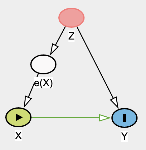
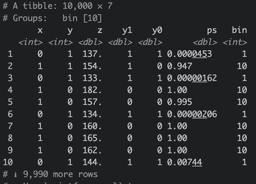
We essentially want to model X from Z to give rise to propensity score of X (e(X)), we shall use logistic regression for this. And then cut e(X), our in case, ps variable, into 10 bins.

ps <- glm(x ~ z, family = "binomial")

df_ps <-
tibble(x,y,z) |>
  mutate(
    y1 = case_when(
      x == 1 ~ y,
      T ~ NA_integer_
    ),
    y0 = case_when(
      x == 0 ~ y,
      T ~ NA_integer_
    ),
    ps = predict(ps,newdata=tibble(z=z), type = "response")) |>
  mutate(bin = cut(ps, 10, labels = F),
         bin_interval = cut(ps, 10)) 

Now let’s group by bin and then estimate our mean outcome for both treatment and control, like so

df_ps |>
  group_by(bin) |>
  mutate(
    y1 = case_when(
      is.na(y1) ~ mean(y1, na.rm = T),
      T ~ y1
    ),
    y0 = case_when(
      is.na(y0) ~ mean(y0, na.rm = T),
      T ~ y0
    )
  ) |> view()

Let’s then ungroup them and calculate ATE.

ATE

df_ps |>
  group_by(bin) |>
  mutate(
    y1 = case_when(
      is.na(y1) ~ mean(y1, na.rm = T),
      T ~ y1
    ),
    y0 = case_when(
      is.na(y0) ~ mean(y0, na.rm = T),
      T ~ y0
    )
  ) |>
  ungroup() |>
  summarize(ate = mean(y1)-mean(y0))

## # A tibble: 1 × 1
##     ate
##   <dbl>
## 1 0.123

Not too shabby! Quite close to the g-estimation ATE! Let’s take a look at CATE as well.

CATE

df_ps |>
  group_by(bin_interval) |>
  mutate(
    y1 = case_when(
      is.na(y1) ~ mean(y1, na.rm = T),
      T ~ y1
    ),
    y0 = case_when(
      is.na(y0) ~ mean(y0, na.rm = T),
      T ~ y0
    )
  ) |>
  summarize(cate = mean(y1)-mean(y0))

## # A tibble: 10 × 2
##    bin_interval    cate
##    <fct>          <dbl>
##  1 (-0.001,0.1] 0.00826
##  2 (0.1,0.2]    0.166  
##  3 (0.2,0.3]    0.287  
##  4 (0.3,0.4]    0.370  
##  5 (0.4,0.5]    0.515  
##  6 (0.5,0.6]    0.587  
##  7 (0.6,0.7]    0.532  
##  8 (0.7,0.8]    0.741  
##  9 (0.8,0.9]    0.797  
## 10 (0.9,1]      0.148

Notice how the CATE is different across all strata? It doesn’t look too helpful for stratum 1 and 10. Looks like the most helpful in stratum 9.

df_ps |>
  group_by(bin_interval) |>
  mutate(
    y1 = case_when(
      is.na(y1) ~ mean(y1, na.rm = T),
      T ~ y1
    ),
    y0 = case_when(
      is.na(y0) ~ mean(y0, na.rm = T),
      T ~ y0
    )
  ) |>
  filter(bin == 9) |>
  group_by(x) |>
  ggplot(aes(x=as.factor(x),y=z)) +
  geom_boxplot(alpha=0.5) +
  geom_jitter(alpha=0.5) +
  ggpubr::stat_compare_means() +
  theme_minimal()

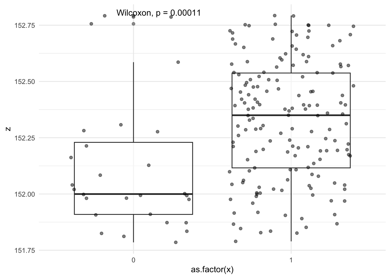
When we visualize Z (blood pressure) with x (treatment groups), looks like the median blood pressure between both groups has a difference of ~0.4 mm Hg, even though if we were to use t test or wilcoxan rank, it will be “statisticall significant”, but clinically it’s really not that different and these two groups stratified by propensity of treatment may give us a true estimate of CATE in this stratum.

Notice how we didn’t model this with glm at all and we’re basically stratified 10 groups from the propensity of treatment. This “stratification” is a form os “adjustment”, or should I say is “adjustment”. We basically trying to reduce / minimize variation of the variable, in this case “propensity of treatment”.

Cheat Sheet

I found this article Causal inference and effect estimation using observational data is super concise and helpful!

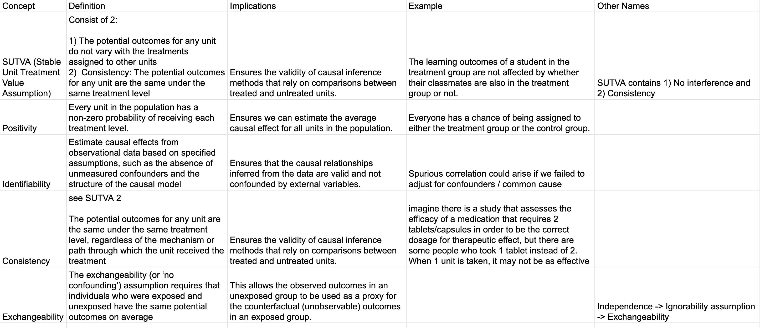
Google sheet. I will continue to revise these for accuracy.

Things We Can Improve on:

• All the above only estimated single point. We can greatly improve our understanding of uncertainty by bootstrapping to get the 95% confidence interval of ATE, CATE and coefficients.
• Our PSS contained stratum 1 and 10 which essentially has very little variation and almost always favors 0 or 1 for treatment propensity, one could trim the edges of propensity scores to get a more realistic ATE and CATE.
• Did I get some of these wrong? Please drop a comment or send me a message, and educate me!

Lessons learnt

• SPICE, the fundation of causal inference. I think I have a better understanding of the assumptions behind CI. I do feel quite a few of the above examples are not too satisfying, but this will do for now and use this as a framework to build further.
• SUTVA teaches us that our treatment cannot influence control group and also has to be consistent (treatment cannot vary).
• Positivity assumption: P(Treatment|Confounder) cannot be ZERO ! Otherwise there is no variation.
• Identifiability: Basically we have to ensure confounders are all adjusted for in order to identify the relationship of interest.
• Consistency is SUTVA 2
• Exchangeability (or ‘no confounding’) assumption requires that individuals who were exposed and unexposed have the same potential outcomes on average

If you like this article:

• please feel free to send me a comment or visit my other blogs
• please feel free to follow me on twitter, GitHub or Mastodon
• if you would like collaborate please feel free to contact me