Exploring Causal Discovery with gCastle through Reticulate in R

Get ready for a thrill ride in causal discovery! We’re diving into gCastle, a Python package, right in R to amp up our skills. Let’s orchestrate our prior knowledge and nail that true DAG. 🔥

As I delve into Aleksander Molak’s Causal Inference and Discovery in Python, I’m increasingly struck by the wealth of talent and intelligence out there focused on enhancing causal inference methodology. I can’t resist giving this a try myself. As someone who has converted to R, I figured, why not tackle this in RStudio using the powerful capabilities of Reticulate? Let’s dive in!

This is going to be an interesting journey, as I’ve recently learned some basics of graph theory that I hope will deepen my understanding of causal discovery, also known as structural equation learning.

Objectives

• Install and load specific modules
• Simulate straight-forward linear continous data structure
• DAG it out
  • write a function to change dagitty object to adjency matrix
  • write a function to plot heatmap of causal matrix
• How to interpret adjency matrix
• The 4 Causal Discovery (CD) Methods
  • Constraint-based method
    • How does it work?
  • Score-based method
  • Functional method
  • Gradient-based method
  • All Results Visualized
• Table of other methods
• Let’s add another collider node and make DAG a tad more complicated
  • Re-run all 4 CD methods
  • Using prior knowledge, only in PC
• Things I need to read up and explore
• Lessons learnt

Install and load specific modules

library(reticulate)
library(tidyverse)
library(ggpubr)
library(dagitty)
library(broom)

# installation
# py_install("gcastle==1.0.3", pip = T)
# py_install("torchvision"), apparently the algorithm requires Torch

gc <- import("castle")
algo <- import("castle.algorithms")

Simulate straight-forward linear continous data structure

set.seed(1)
n <- 10000
a <- rnorm(n) 
b <- rnorm(n) 
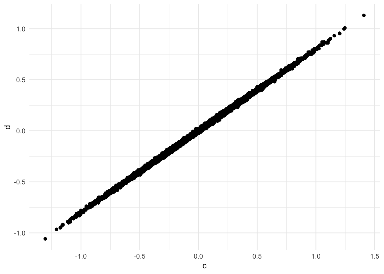
c <- 0.3*a + 0.2*b + 0.01*rnorm(n)
d <- 0.8*c + 0.01*rnorm(n)
# e <- -0.4*a + -0.4*d + 0.01*rnorm(n) # we will add a collider later

df <- data.frame(a,b,c,d)

df1 <- as.matrix(df)

df |>
  ggplot(aes(x=c,y=d)) +
  geom_point() +
  theme_minimal()

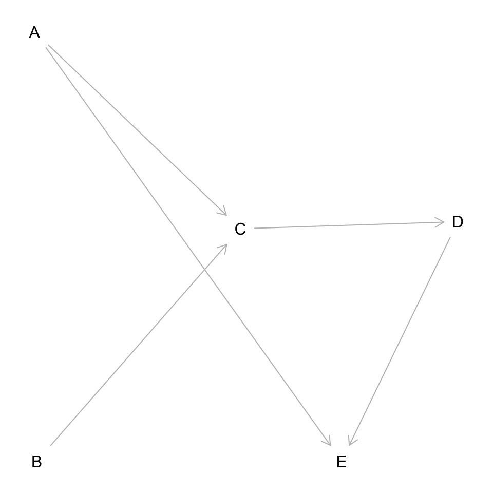
DAG it out

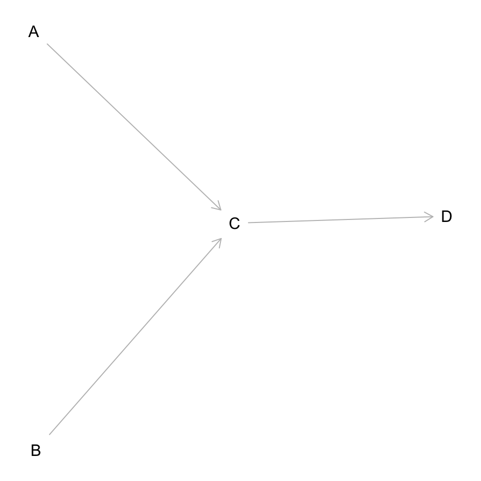
dag <- dagitty('dag {
bb="0,0,1,1"
A [pos="0.236,0.380"]
B [pos="0.238,0.561"]
C [pos="0.413,0.463"]
D [pos="0.600,0.460"]
A -> C
B -> C
C -> D
}'
)

plot(dag)

write a function to change dagitty object to adjacency matrix

I’ve directly copied this from orientDAG. For some reason, this package isn’t available for RStudio 4+—or maybe it’s not on CRAN; I’m not entirely sure. 🤷‍♂️ Regardless, having the adjacency information will be invaluable for constructing heatmaps for comparison.

dagitty_to_adjmatrix <- function(daggity_obj) {
  edg <- dagitty:::edges(daggity_obj)
  node_names <- dagitty:::names.dagitty(daggity_obj)
  ans_mat <- matrix(
    data = 0, nrow = length(node_names),
    ncol = length(node_names),
    dimnames = list(node_names, node_names)
  )

  ans_mat[as.matrix(edg[c("v", "w")])] <- 1
  return(ans_mat)
}

dag_true <- dagitty_to_adjmatrix(dag)

dag_true

##   A B C D
## A 0 0 1 0
## B 0 0 1 0
## C 0 0 0 1
## D 0 0 0 0

write a function to plot heatmap of causal matrix

hm <- function(x,title,dag_true=F) {
  if (dag_true) {
    color <- "green"
  } else { color <- "blue"}
  g <- as_tibble(x) 
  num_nodes <- nrow(x)
  colname_g <- c(paste0("V",1:num_nodes))
  colnames(g) <- colname_g
  
  g1 <- g |>
  mutate(Var2 = row_number()) |>
  pivot_longer(cols = colname_g, names_to = "Var1", values_to = "Freq") |>
  mutate(Var1 = case_when(
    str_detect(Var1, "V") ~ str_extract(Var1,"[1-9]")))  |>
  ggplot(aes(x=Var1,y=Var2)) +
  geom_tile(aes(fill=Freq), color = "black", alpha=0.5) +
  scale_fill_gradient(low = "white", high = color) +
  theme_minimal() +
  scale_y_reverse() +
  theme(legend.position = "none", panel.grid.major = element_blank(), panel.grid.minor = element_blank()) +
  ggtitle(label = title)

  return(g1)
}

How to interpret Adjacency Matrix

dag_true

##   A B C D
## A 0 0 1 0
## B 0 0 1 0
## C 0 0 0 1
## D 0 0 0 0

row (usually represented by i) -> column (usually represented by j).
In this case, A -> C, should have a 1 on [A,C] or [1,3].
B -> C, should have a 1 on [B,C] or [2,3].
C -> D, should have a 1 on [C,D] or [3,4].

The adjacency matrix above represents our true DAG. Now, if for some reason there is an undirected edge in the DAG, for example between nodes B and C, then the entries at [2,3] and [3,2] in the adjacency matrix would both be 1.

Constraint-based: Peter Clark (PC) Algorithm

The PC algorithm, named after its creators Peter Spirtes and Clark Glymour, is built on a statistical framework that assumes a set of observed variables and aims to discover causal directions based on conditional independence tests. Starting with a fully connected, undirected graph, the PC algorithm iteratively removes edges that are deemed unnecessary for explaining the observed correlations or dependencies among variables. Then, the algorithm aims to orient the remaining edges to establish a likely causal order.

pc <- algo$PC()

pc$learn(data = df1)

pc_mat <- pc$causal_matrix

pc_g <- hm(pc_mat, "PC")
true_g <- hm(dag_true, "true_dag",T)

ggarrange(pc_g,true_g)

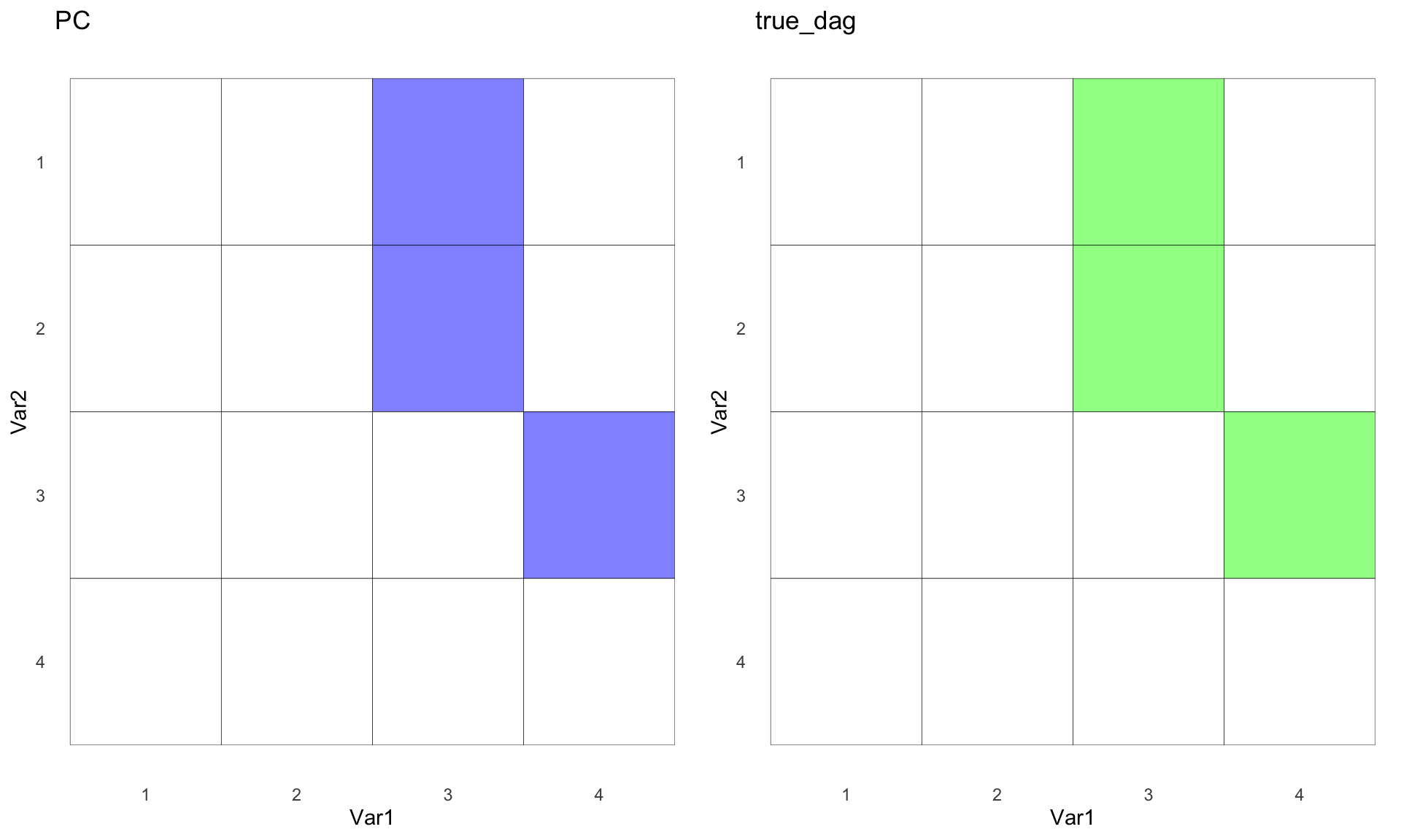
Wow, impressive! PC managed to uncover the true DAG. Let’s dive into how PC actually works.

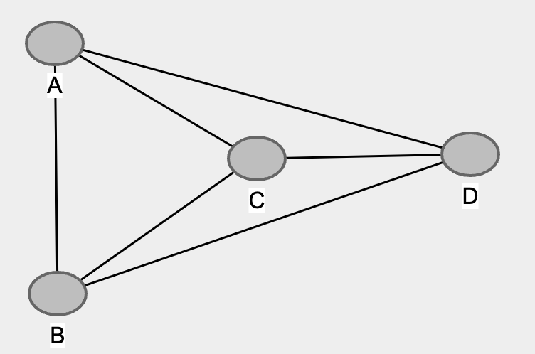
How does it work? 👍

1. Connect all nodes
2. Remove edges from nodes with unconditional independence
3. Remove edges from nodes with conditional independence
4. Direct the edges of collider
5. Complete the direction of the nodes

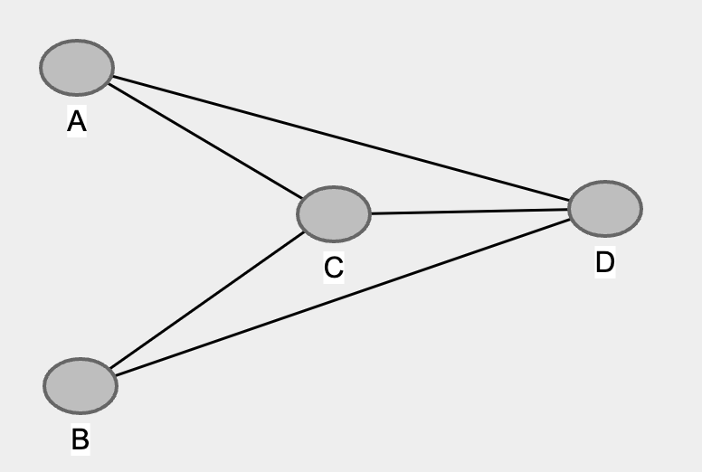
1. Connect all nodes 🕷️

2. Remove edges from nodes with unconditional independence ✄

We will use Pearson correlation to tease this out and use 0.01 as a threshold.

cor(df)

##             a           b         c         d
## a 1.000000000 0.004845078 0.8379534 0.8377377
## b 0.004845078 1.000000000 0.5490910 0.5483710
## c 0.837953423 0.549091040 1.0000000 0.9994109
## d 0.837737692 0.548371035 0.9994109 1.0000000

cor(df) < 0.01

##       a     b     c     d
## a FALSE  TRUE FALSE FALSE
## b  TRUE FALSE FALSE FALSE
## c FALSE FALSE FALSE FALSE
## d FALSE FALSE FALSE FALSE

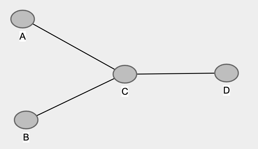
As we can see A and B are unconditionally independent. Hence we will remove the edge between A and B like so…

3. Remove edges from nodes with conditional independence ✄

Now it’s time to delve into some simple partial correlation or linear regression to sort this out. We’ll be using our trusty tool, linear regression. Since we know that A and B are not connected, the connection must lie with C, D, or both. Let’s find out which edge we can eliminate by checking for conditional independence.

Let’s look at A ~ C + D. Which node coefficient will lose its significance? Let’s find out!

# check A and D, given C
lm(a~d+c,df) |> tidy()

## # A tibble: 3 × 5
##   term         estimate std.error statistic  p.value
##   <chr>           <dbl>     <dbl>     <dbl>    <dbl>
## 1 (Intercept) -0.000136   0.00553   -0.0247 0.980   
## 2 d            0.821      0.553      1.48   0.138   
## 3 c            1.68       0.443      3.79   0.000154

Nice! Looks like D lost its statistical significance when controlled for C. This means, the edge from A to D can be removed because A and D are now independent when C is adjusted. Let’s now look at B.

# check B and D, given C
lm(b~d+c,df) |> tidy()

## # A tibble: 3 × 5
##   term         estimate std.error statistic  p.value
##   <chr>           <dbl>     <dbl>     <dbl>    <dbl>
## 1 (Intercept) -0.000179   0.00828   -0.0216 0.983   
## 2 d           -1.15       0.829     -1.38   0.167   
## 3 c            2.41       0.664      3.64   0.000278

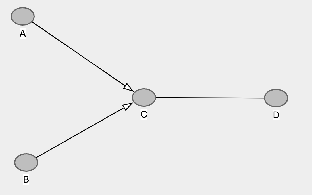
Superb! Remove edge from B to D it is. And now it should look like…

4. Direct the edges of collider 🎬

Still with me? We’re almost there! Next up: identifying the collider, also known as a v-structure. This is crucial because a collider can turn an independent relationship between two nodes into a dependent one when adjusted. Based on the given graph, a good guess for the collider might be A -> C <- B. Why not A -> C <- D or B -> C <- D? Well, we just found out that the relationships between A and D, as well as B and D, become independent when C is controlled. So, it must be something like A -> C -> D or A <- C <- D, etc.

If A -> C <- B is indeed a collider, then A and B would become dependent when we control for C. Let’s inspect!

lm(a~b+c,df) |> tidy()

## # A tibble: 3 × 5
##   term         estimate std.error statistic p.value
##   <chr>           <dbl>     <dbl>     <dbl>   <dbl>
## 1 (Intercept) -0.000259  0.000336    -0.770   0.441
## 2 b           -0.666     0.000405 -1642.      0    
## 3 c            3.33      0.00111   3013.      0

Perfecto! It works! B coefficient is now significant !!! The magic of collider. This also means we can direct the edges like so…

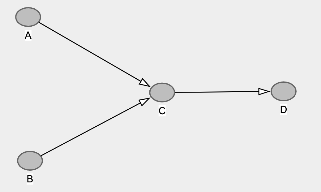
5. Complete the direction of the nodes

Since we know A -> C <- D is not a collider, the edge arrow must be directing from C to D. Hence, we’re back to our complete DAG! ✅

Score-based: Greedy Equivalence Search (GES) 🔍

Greedy Equivalence Search (GES) is a statistical algorithm used for learning the structure of Bayesian networks from observational data. The algorithm consists of two main phases: the forward, or “greedy,” phase where edges are added to maximize a scoring function, and the backward, or “equivalence,” phase where unnecessary edges are removed while maintaining the same likelihood score. GES aims to find an equivalence class of Bayesian networks that have the same observational distributions, offering a balance between computational efficiency and accuracy in identifying causal relationships among variables.

ges <- algo$GES(criterion = "bic")

ges$learn(data = df1)

ges_mat <- ges$causal_matrix

ges_g <- hm(ges_mat, "GES")

ggarrange(ges_g,true_g)

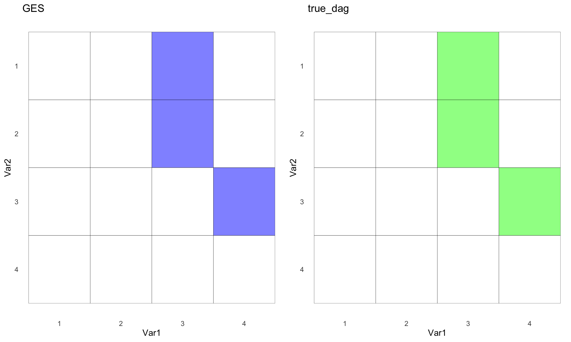
Not too shabby. GES recovered the true DAG. Way to go! ✅

Functional: Linear Non-Gaussian Acyclic Model (LINGAM)

LiNGAM unlike traditional linear models that often assume Gaussian distributions, LiNGAM operates under the assumption that the data is generated from non-Gaussian sources, allowing it to identify causal directions even in the presence of linear relationships. It builds acyclic causal models by leveraging the distinct statistical properties of non-Gaussian distributions, providing a more nuanced understanding of the underlying causal structure among the variables being studied.

lingam <- algo$ICALiNGAM()

lingam$learn(data = df1)

lingam_mat <- lingam$causal_matrix

lingam_g <- hm(lingam_mat, "LINGAM")
ggarrange(lingam_g,true_g)

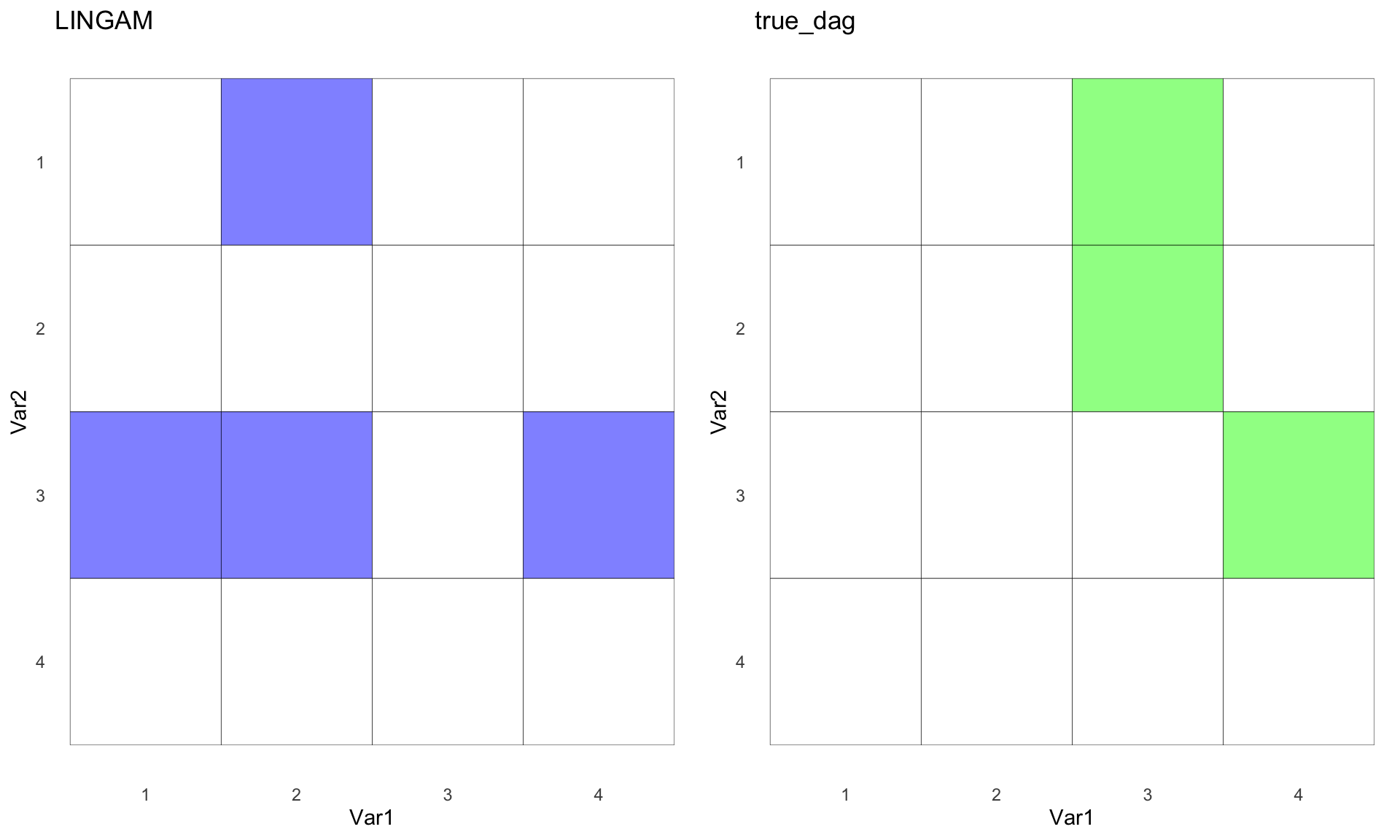
Hmmm, not the result we were hoping for, right? Our structure is in normal form, so maybe that’s why it’s not working as expected. 🤷‍♂️ Clearly, I have more reading and learning to do. When you think about it, real-life data is often non-normal, so maybe these methods will shine in those settings. I have a lot to learn, and I’m considering dedicating another blog post to more advanced methods, perhaps using more realistic simulated data. Stay tuned!

Ooo… Adjacency Matrix With Actual Coefficient! ❤️

lingam$weight_causal_matrix

##          [,1]      [,2] [,3]      [,4]
## [1,] 0.000000 -1.496010    0 0.0000000
## [2,] 0.000000  0.000000    0 0.0000000
## [3,] 2.332736  4.986864    0 0.7998635
## [4,] 0.000000  0.000000    0 0.0000000

I really like this. More fine-tuned estimates to assess the situation. Definitely a good tool!

Gradient-based method: NOTEARS ❌😭i

NOTEARS employs continuous optimization techniques to fit the DAG. Specifically, it uses gradient descent methods to minimize a loss function subject to acyclicity constraints, which are ingeniously encoded to be differentiable. This results in a more efficient and scalable algorithm, making NOTEARS suitable for handling larger datasets and high-dimensional problems in causal inference.

notear <- algo$Notears()

notear$learn(df1)

notear_mat <- notear$causal_matrix
# notear$weight_causal_matrix <- this also has weighted causal/adjacency matrix ❤️

notear_g <- hm(notear_mat,"NOTEARS")

ggarrange(notear_g,true_g)

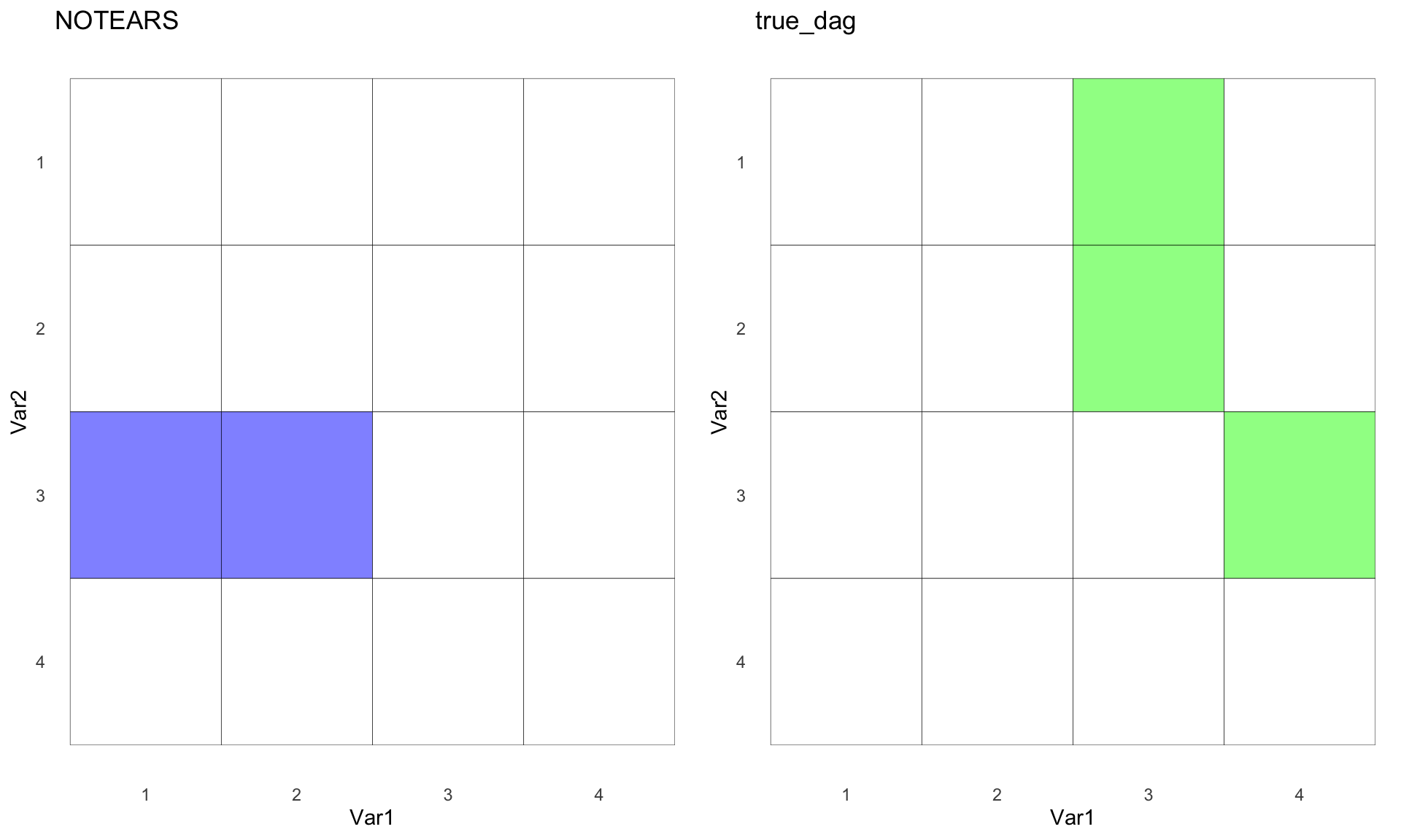
Oops! The method sounded cool 😎, but the results? Not so much 🤣. This just goes to show that understanding the underlying causal assumptions of the DAG is crucial before diving into any of these techniques.

There is a shiny app called Causal Disco 🪩 that you can apply the assumptions and then it shows what algorithm is best for those. Pretty cool. Though it doesn’t have gCastle or Causal-learn. Lol, why would they, it’s no R. Again, advocate to learn both R + Python!

All 4 CD Methods

ggarrange(pc_g,ges_g,true_g,lingam_g,notear_g)

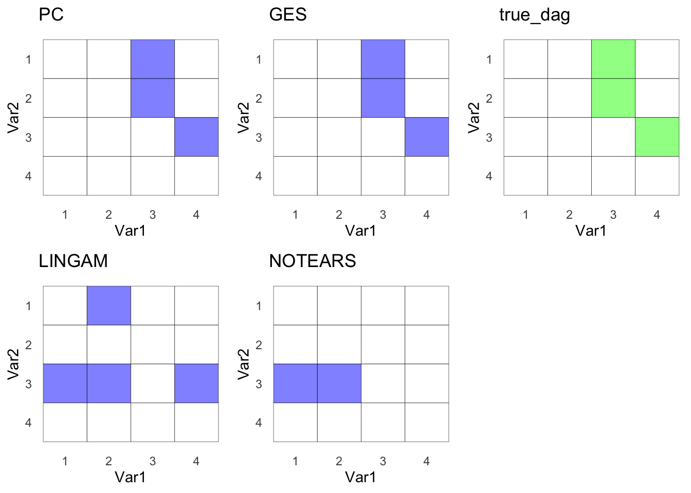
Table of other methods

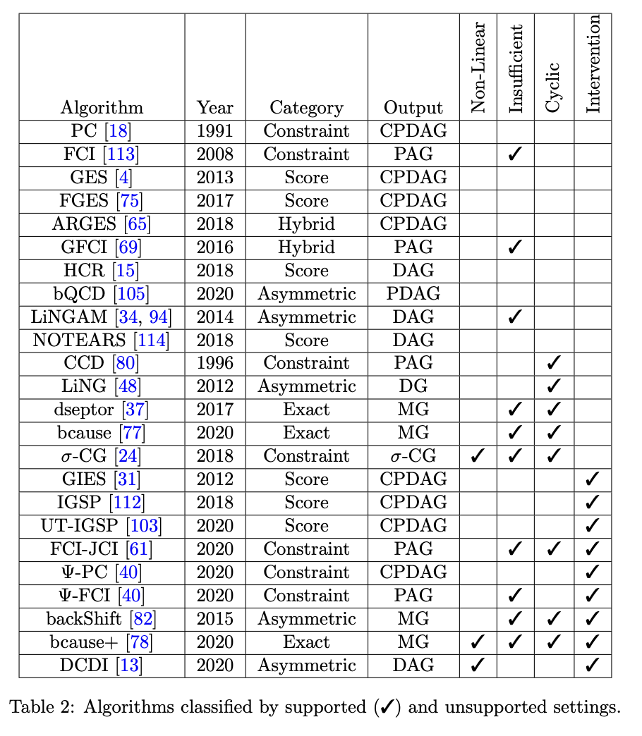A Survey on Causal Discovery:Theory and Practice - Alessio Zanga and Fabio Stella.

This article is great! Easy to follow and good flow. Highly recommended!

Let’s add another collider node E and make DAG a tad more complicated

set.seed(1)
n <- 10000
a <- rnorm(n) 
b <- rnorm(n) 
c <- 0.3*a + 0.2*b + 0.01*rnorm(n)
d <- 0.8*c + 0.01*rnorm(n)
e <- -0.4*a + -0.4*d + 0.01*rnorm(n) # we will add a collider later

df <- data.frame(a,b,c,d,e)

df1 <- as.matrix(df)

dag <- dagitty('dag {
bb="0,0,1,1"
A [pos="0.236,0.380"]
B [pos="0.238,0.561"]
C [pos="0.413,0.463"]
D [pos="0.600,0.460"]
E [pos="0.5,0.561"]
A -> C
B -> C
C -> D
A -> E
D -> E
}'
)

plot(dag)

dag_true <- dagitty_to_adjmatrix(dag)

# PC
pc <- algo$PC()
pc$learn(data = df1)
pc_mat <- pc$causal_matrix
pc_g <- hm(pc_mat, "PC")
true_g <- hm(dag_true, "true_dag",T)

#GES
ges <- algo$GES(criterion = "bic")
ges$learn(data = df1)
ges_mat <- ges$causal_matrix
ges_g <- hm(ges_mat, "GES")

#lingam
lingam <- algo$ICALiNGAM()
lingam$learn(data = df1)
lingam_mat <- lingam$causal_matrix
lingam_g <- hm(lingam_mat, "LINGAM")

#notears
notear <- algo$Notears()
notear$learn(df1)
notear_mat <- notear$causal_matrix
notear_g <- hm(notear_mat,"NOTEARS")

Observe that this DAG is not the same as the one before. There was an added E collider from A and D.

Re-run all 4 CD methods

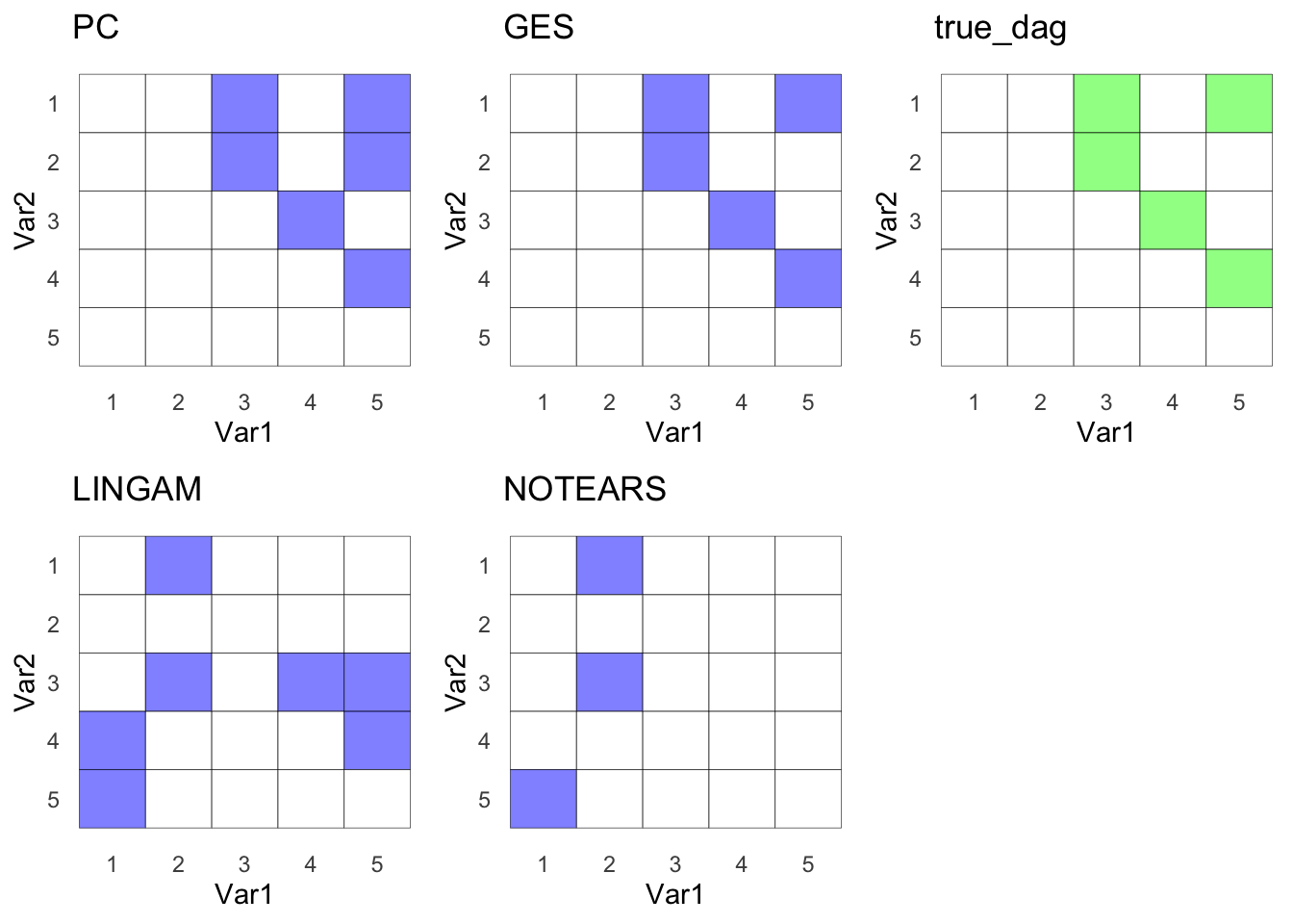
Wow, intriguing! It appears that PS and GES come closer to the true DAG than LiNGAM and NOTEARS. We’ll delve into the scenarios where LiNGAM and NOTEARS excel in a future post. Remember, these are all tools; the key is knowing when to use each one effectively.

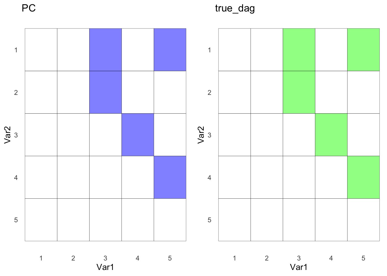
Using prior knowledge, only in PC

Assuming that we know the there is no edge from B and E, we can supply this on prior knowledge.

prior <- gc$common$priori_knowledge$PrioriKnowledge

# create how many nodes
priori <- prior(n_nodes=5L)
priori$matrix

##      [,1] [,2] [,3] [,4] [,5]
## [1,]    0   -1   -1   -1   -1
## [2,]   -1    0   -1   -1   -1
## [3,]   -1   -1    0   -1   -1
## [4,]   -1   -1   -1    0   -1
## [5,]   -1   -1   -1   -1    0

The naive prior knowledge looks like this. 👆.
-1 means can be modified.
0 means do not assign and don’t modify.
1 means assigned and don’t modify.

# Remove edge from B to E in both directions, remember this is python, they start at 0th, hence the 1 and 4.
priori$add_forbidden_edge(i = 1L,j = 4L)
priori$add_forbidden_edge(i = 4L,j = 1L)
priori$matrix

##      [,1] [,2] [,3] [,4] [,5]
## [1,]    0   -1   -1   -1   -1
## [2,]   -1    0   -1   -1    0
## [3,]   -1   -1    0   -1   -1
## [4,]   -1   -1   -1    0   -1
## [5,]   -1    0   -1   -1    0

Let’s rerun PC algorithm with the prior knowledge, knowing B and E are not connected.

pc <- algo$PC(priori_knowledge=priori)
pc$learn(data = df1)
pc_mat <- pc$causal_matrix
pc_g <- hm(pc_mat, "PC")
ggarrange(pc_g,true_g)

Wow, that’s quite a journey, isn’t it? But we’ve learned so much and it’s been invigorating! A big thank you to Aleksander Molak for such an insightful book. It took me multiple reads of the Causal Discovery section just to scratch the surface, but it’s been so rewarding. I have to say, it’s right up there with ‘The Book of Why’ by Judea Pearl in terms of awesomeness. If you haven’t read it yet, I highly recommend you do. I know I’ll be going back to both books for reference!

Things to learn and improve on:

• Try to do GES step-by-step
• Going to give PyWhy: Causal Learn a try. It looks really cool and has all of the algorithms gCastle has, has more flexibility in parameters, and best of all it’s part of PyWhy. Will blog about this next time.
• Need to add metrics next time to assess their F1, accuracy, etc.
• Need to get some other non-Gaussian dataset to experiment with these tools. Ideas and guidance welcomed!

Lessons learnt:

• scale_y_reverse reverses the y axis display
• Learnt how to do PC step by step on simple linear continuous data
• gCastle is quite easy and friendly to use, even in R
• All 4 CD tools (Constraint, Score-based, Functional, and Gradient-based)
• A great article that has more in depth information of other tools that I will keep referring to. link
• Found Causal-learn. Great API documentation, great people as well on discord.

If you like this article:

• please feel free to send me a comment or visit my other blogs
• please feel free to follow me on twitter, GitHub or Mastodon
• if you would like collaborate please feel free to contact me