Exploring Causal Discovery with Causal-learn and Reticulate in R
By Ken Koon Wong in r R reticulate causal discovery structural equation learning causal-learn causallearn python pywhy
August 27, 2023
The PyWhy Causal-learn Discord community is fantastic! The package documentation is equally impressive, making experiential learning both fun and informative. Truly, it’s another exceptional tool for causal discovery at our fingertips! ❤️
It’s time to delve into
PyWhy’s Causal-learn! his brief blog post leverages the framework from a previous blog to navigate through DAGs using causal-learn rather than gCastle. If you’re keen on a more in-depth exploration of the PC algorithm, be sure to check out the
previous blog.
Objectives
- Install and load specific modules
- Simulate straight-forward linear continous data structure
- DAG it out
- Slight difference in adjency matrix
- All 4 Results Visualized
- Let’s add another collider node and make DAG a tad more complicated
- Final Thoughts
- Lessons learnt
Install and load specific modules
library(reticulate)
library(tidyverse)
library(dagitty)
library(ggpubr)

# installation
# py_install("causal-learn",pip=T)
Simulate straight-forward linear continous data structure
set.seed(1)
n <- 1000
a <- rnorm(n)
b <- rnorm(n)
c <- 0.3*a + 0.2*b + 0.01*rnorm(n)
d <- 0.8*c + 0.01*rnorm(n)
# e <- -0.4*a + -0.4*d + 0.01*rnorm(n) # we will add a collider later

df <- data.frame(a,b,c,d)
df1 <- as.matrix(df)
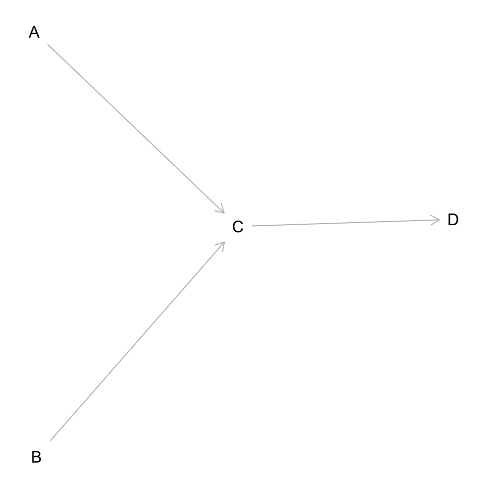
DAG it out
dag <- dagitty('dag {
bb="0,0,1,1"
A [pos="0.236,0.380"]
B [pos="0.238,0.561"]
C [pos="0.413,0.463"]
D [pos="0.600,0.460"]
A -> C
B -> C
C -> D
}'
)

plot(dag)
Create functions
dagitty_to_adjmatrix <- function(daggity_obj) {
  edg <- dagitty:::edges(daggity_obj)
  node_names <- dagitty:::names.dagitty(daggity_obj)
  ans_mat <- matrix(
    data = 0, nrow = length(node_names),
    ncol = length(node_names),
    dimnames = list(node_names, node_names)
  )

  ans_mat[as.matrix(edg[c("v", "w")])] <- 1
  return(ans_mat)
}

dag_true <- dagitty_to_adjmatrix(dag)

hm <- function(x,title,dag_true=F) {
  if (dag_true) {
    color <- "green"
  } else { color <- "blue"}
  g <- as_tibble(x)
  num_nodes <- nrow(x)
  colname_g <- c(paste0("V",1:num_nodes))
  colnames(g) <- colname_g

  g1 <- g |>
  mutate(Var2 = row_number()) |>
  pivot_longer(cols = colname_g, names_to = "Var1", values_to = "Freq") |>
  mutate(Var1 = case_when(
    str_detect(Var1, "V") ~ str_extract(Var1,"[1-9]")))  |>
  ggplot(aes(x=Var1,y=Var2)) +
  geom_tile(aes(fill=Freq), color = "black", alpha=0.5) +
  geom_text(aes(x=Var1,y=Var2,label=round(Freq, digits = 2))) +
  scale_fill_gradient(low = "white", high = color, limits = c(0,5), na.value = "white") + #to adjust for causal-learn's adj matrix method
  theme_minimal() +
  scale_y_reverse() +
  theme(legend.position = "none", panel.grid.major = element_blank(), panel.grid.minor = element_blank()) +
  ggtitle(label = title)

  return(g1)
}

true_dag <- dagitty_to_adjmatrix(dag)
dag_g <- hm(true_dag, "True DAG", dag_true=T)
As before, we’ve created a function to convert the DAG class to an adjacency matrix for convenience. The code for the heatmap has been updated as well. Causal-learn offers a slightly different approach, adding flexibility to their adjacency matrix representation. As a result, I’ve included an additional limit parameter in the scale_fill_gradient function.
Slight difference in adjency matrix
Recall on our previous blog, i -> j is represented as [i,j] = 1. But in Causal-learn, there is -1 in addition.
For example:
A -> C would be [A,C] = -1 and [C,A] = 1.
C -> D would be [C,D] = -1 and [C,D] = 1.
A tip from Bryan @
Discord PyWhy gave a tip that -1 represents arrowtail and 1 represents arrowhead. 😀
With that in mind, let’s maintain consistency with the previous blog by using the same adjacency matrix format. To that end, the function above has been modified to mask any numbers less than zero, while still displaying the actual value. Later on, we’ll transpose the matrix to align with the format we’re accustomed to. 😎
All 4 CD Methods and more
# load causallearn
algo <- import("causallearn.search")

# Constrained
# pc
pc <- algo$ConstraintBased$PC
pc1 <- pc$pc(data = df1)
# adjacency matrix
pc_mat <- pc1$G$graph
pc_g <- hm(pc_mat |> t(),"PC")

# FCI
fci <- algo$ConstraintBased$FCI$fci
fci1 <- fci(dataset=df1) #instad of data, this uses dataset instead
fci_mat <- fci1[[1]]$graph |> t()
fci_g <- hm(fci_mat, "FCI")

#Score base
#GES
ges <- algo$ScoreBased$GES$ges
ges1 <- ges(df1)
ges_g <- hm(ges1$G$graph |> t(),"GES")

#Exact
exact <- algo$ScoreBased$ExactSearch$bic_exact_search
exact_mat <- exact(df1)[[1]]
exact_g <- hm(exact_mat, "Exact")

#Functional
#lingam
lingam <- algo$FCMBased$lingam$ICALiNGAM()
lingam$fit(X = df1)
lingam_mat <- lingam$adjacency_matrix_ |> t()
lingam_g <- hm(lingam_mat, "LINGAM")


# Hidden causal representation learning
# generalized independent noise (GIN)
gin <- algo$HiddenCausal$GIN$GIN$GIN
gin1 <- gin(df1)
gin_mat <- gin1[[1]]$graph
gin_g <- hm(gin_mat, "GIN")

# Permutation-based causal discovery methods
#GRaSP
gp <- algo$PermutationBased$GRaSP$grasp
gp1 <- gp(df1)
gp_mat <- gp1$graph |> t()
gp_g <- hm(gp_mat, "GRaSP")

ggarrange(dag_g,pc_g,fci_g,ges_g,exact_g,lingam_g,gin_g,gp_g)
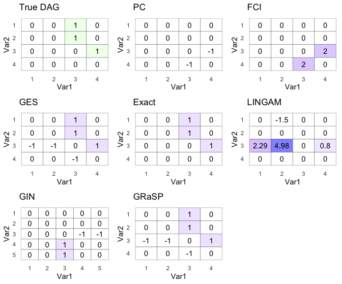
Wow, not bad. GES, Exact, and GRaSP got the DAG right!
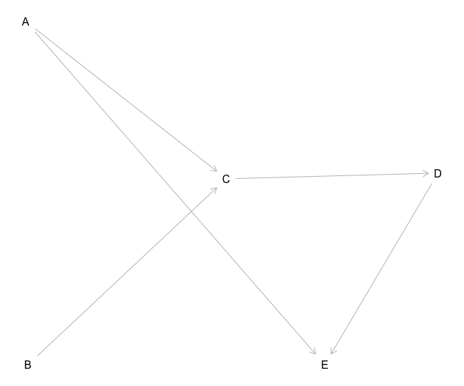
Let’s add another collider node E and make DAG a tad more complicated
set.seed(1)
n <- 1000
a <- rnorm(n)
b <- rnorm(n)
c <- 0.3*a + 0.2*b + 0.01*rnorm(n)
d <- 0.8*c + 0.01*rnorm(n)
e <- -0.4*a + -0.4*d + 0.01*rnorm(n) # we will add a collider later

df <- data.frame(a,b,c,d,e)
df1 <- as.matrix(df)

#dag
dag <- dagitty('dag {
bb="0,0,1,1"
A [pos="0.236,0.380"]
B [pos="0.238,0.561"]
C [pos="0.413,0.463"]
D [pos="0.600,0.460"]
E [pos="0.5,0.561"]
A -> C
B -> C
C -> D
D -> E
A -> E
}'
)

plot(dag)
true_dag <- dagitty_to_adjmatrix(dag)
dag_g <- hm(true_dag, "True DAG", dag_true=T)

# Causal discovery
# Constrained
# pc
pc <- algo$ConstraintBased$PC
pc1 <- pc$pc(data = df1)
# adjacency matrix
pc_mat <- pc1$G$graph
pc_g <- hm(pc_mat |> t(),"PC")

# FCI
fci <- algo$ConstraintBased$FCI$fci
fci1 <- fci(dataset=df1) #instad of data, this uses dataset instead
fci_mat <- fci1[[1]]$graph |> t()
fci_g <- hm(fci_mat, "FCI")

#Score base
#GES
ges <- algo$ScoreBased$GES$ges
ges1 <- ges(df1)
ges_g <- hm(ges1$G$graph |> t(),"GES")

#Exact
exact <- algo$ScoreBased$ExactSearch$bic_exact_search
exact_mat <- exact(df1)[[1]]
exact_g <- hm(exact_mat, "Exact")

#Functional
#lingam
lingam <- algo$FCMBased$lingam$ICALiNGAM()
lingam$fit(X = df1)
lingam_mat <- lingam$adjacency_matrix_ |> t()
lingam_g <- hm(lingam_mat, "LINGAM")


# Hidden causal representation learning
# generalized independent noise (GIN)
gin <- algo$HiddenCausal$GIN$GIN$GIN
gin1 <- gin(df1)
gin_mat <- gin1[[1]]$graph
gin_g <- hm(gin_mat, "GIN")

# Permutation-based causal discovery methods
#GRaSP
gp <- algo$PermutationBased$GRaSP$grasp
gp1 <- gp(df1)
gp_mat <- gp1$graph |> t()
gp_g <- hm(gp_mat, "GRaSP")

ggarrange(dag_g,pc_g,fci_g,ges_g,exact_g,lingam_g,gin_g,gp_g)
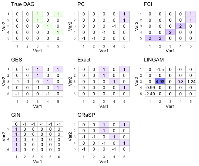 .
.
GES, Exact, and GRaSP won the race again!
Final Thoughts
I’m truly impressed with this community, both for its incredibly informative documentation and its highly responsive Discord channel ❤️. Even when I ask simple questions like ‘How do I get a return of the adjacency matrix?’, I receive prompt answers. What’s more, I appreciate the abundance of methods available, each accompanied by extensive documentation and additional references for further reading.
Lessons Learnt: 👍
Causal-learnis another great tool. I will be using this predominantly from now onwards, unless if I needNOTEARSorautoencoderthen we’ll havegCastlefor that- A variety of adjacency matrix exists, need context
- Another great community that we can ask questions!
- R users really don’t need an R wrapper for all these great python tools 😎
If you like this article:
- please feel free to send me a comment or visit my other blogs
- please feel free to follow me on twitter, GitHub or Mastodon
- if you would like collaborate please feel free to contact me
- Posted on:
- August 27, 2023
- Length:
- 6 minute read, 1106 words
- Categories:
- r R reticulate causal discovery structural equation learning causal-learn causallearn python pywhy