What Happens If Our Model Adjustment Includes A Collider?

Beware of what we adjust. As we have demonstrated, adjusting for a collider variable can lead to a false estimate in your analysis. If a collider is included in your model, relying solely on AIC/BIC for model selection may provide misleading results and give you a false sense of achievement.

Let’s DAG out The True Causal Model

# Loading libraries
library(ipw)
library(tidyverse)
library(dagitty)
library(DT)

# Creating the actual/known DAG
dag2 <- dagitty('dag {
bb="0,0,1,1"
W [adjusted,pos="0.422,0.723"]
X [exposure,pos="0.234,0.502"]
Y [outcome,pos="0.486,0.498"]
Z [pos="0.232,0.264"]
collider [pos="0.181,0.767"]
W -> X
W -> Y
X -> Y
X -> collider
Y -> collider
Z -> W
Z -> X
}
')

plot(dag2)

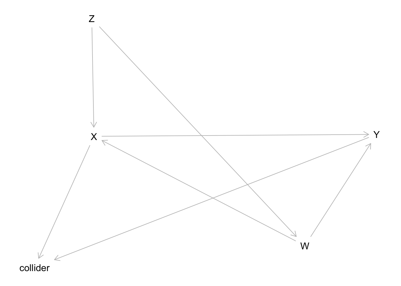
X: Treatment/Exposure variable/node.
Y: Outcome variable/node.
Z: Something… not sure what this is called 🤣.
W: Confounder.
collider: Collider, V-structure.

Let’s find out what is our minimal adjustment for total effect

adjust <- adjustmentSets(dag2)
adjust

## { W }

Perfect! We only need to adjust W. Now we know which node is correct to adjust, let’s simulate data!

set.seed(1)

# set number of observations
n <- 1000
z <- rnorm(n)
w <- 0.6*z + rnorm(n)
x <- 0.5*z + 0.2*w + rnorm(n)
y <- 0.5*x + 0.4*w + rnorm(n) 
collider <- -0.4*x + -0.4*y + rnorm(n) 

# create a dataframe for the simulated data
df <- tibble(z=z,w=w,y=y,x=x, collider=collider)

datatable(df)

Simple Model (y ~ x)

model_c <- lm(y~x, data=df)
summary(model_c)

## 
## Call:
## lm(formula = y ~ x, data = df)
## 
## Residuals:
##     Min      1Q  Median      3Q     Max 
## -3.8671 -0.7063 -0.0466  0.7757  3.1475 
## 
## Coefficients:
##             Estimate Std. Error t value Pr(>|t|)    
## (Intercept)  0.00651    0.03585   0.182    0.856    
## x            0.68853    0.02840  24.244   <2e-16 ***
## ---
## Signif. codes:  0 '***' 0.001 '**' 0.01 '*' 0.05 '.' 0.1 ' ' 1
## 
## Residual standard error: 1.134 on 998 degrees of freedom
## Multiple R-squared:  0.3707,	Adjusted R-squared:   0.37 
## F-statistic: 587.8 on 1 and 998 DF,  p-value: < 2.2e-16

Note that our true x coefficient is 0.5. Our current naive model shows 0.6885278

Correct Model (y ~ x + w) ✅

model_cz <- lm(y~x + w, data=df)
summary(model_cz) 

## 
## Call:
## lm(formula = y ~ x + w, data = df)
## 
## Residuals:
##     Min      1Q  Median      3Q     Max 
## -3.2568 -0.7185 -0.0120  0.7166  3.0578 
## 
## Coefficients:
##             Estimate Std. Error t value Pr(>|t|)    
## (Intercept)  0.01703    0.03287   0.518    0.604    
## x            0.51230    0.02900  17.665   <2e-16 ***
## w            0.41600    0.03015  13.797   <2e-16 ***
## ---
## Signif. codes:  0 '***' 0.001 '**' 0.01 '*' 0.05 '.' 0.1 ' ' 1
## 
## Residual standard error: 1.039 on 997 degrees of freedom
## Multiple R-squared:  0.4716,	Adjusted R-squared:  0.4705 
## F-statistic: 444.8 on 2 and 997 DF,  p-value: < 2.2e-16

Not bad ! x coefficient is 0.5123039

Alright, What About Everything Including Collider (y ~ x + z + w + collider) ❌

model_czwall <- lm(y~x + w + collider, data=df)
summary(model_czwall)  

## 
## Call:
## lm(formula = y ~ x + w + collider, data = df)
## 
## Residuals:
##     Min      1Q  Median      3Q     Max 
## -3.1776 -0.6748  0.0032  0.6595  2.7895 
## 
## Coefficients:
##              Estimate Std. Error t value Pr(>|t|)    
## (Intercept)  0.007299   0.030354   0.240     0.81    
## x            0.258613   0.032959   7.846  1.1e-14 ***
## w            0.362523   0.028126  12.889  < 2e-16 ***
## collider    -0.374754   0.028403 -13.194  < 2e-16 ***
## ---
## Signif. codes:  0 '***' 0.001 '**' 0.01 '*' 0.05 '.' 0.1 ' ' 1
## 
## Residual standard error: 0.9593 on 996 degrees of freedom
## Multiple R-squared:  0.5502,	Adjusted R-squared:  0.5488 
## F-statistic: 406.1 on 3 and 996 DF,  p-value: < 2.2e-16

😱 x is now 0.2586135. Not good!

Let’s Visualize All Models

load("df_model.rda")

df_model |>
  mutate(color = case_when(
    str_detect(formula, "collider") ~ 1,
    TRUE ~ 0
  )) |>
  ggplot(aes(x=formula,y=estimate,ymin=lower,ymax=upper)) +
  geom_point(aes(color=as.factor(color))) +
  geom_linerange(aes(color=as.factor(color))) +
  scale_color_manual(values = c("grey","red")) +
  coord_flip() +
  geom_hline(yintercept = 0.5) +
  theme_minimal() +
  theme(legend.position = "none") 

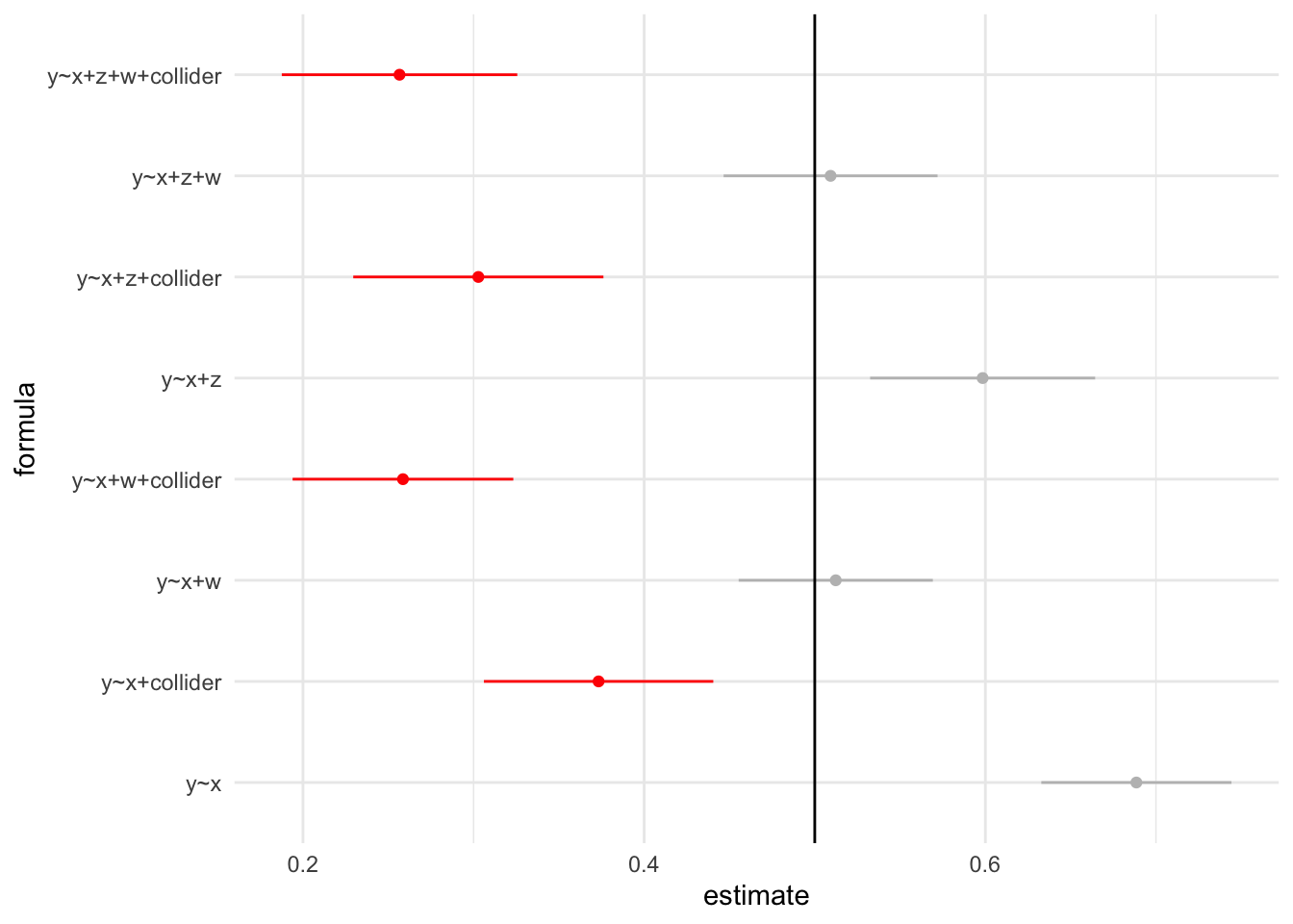
The red lines represent models with colliders adjusted. It’s important to observe that none of these models contain the true value within their 95% confidence intervals. Adjusting for colliders can lead to biased estimates, particularly when the colliders directly affect both the treatment and outcome variables. Careful consideration should be given to the inclusion of colliders in the analysis to avoid potential distortions in the results.”

Let’s check IPW

ipw <- ipwpoint(
  exposure = x,
  family = "gaussian",
  numerator = ~ 1,
  denominator = ~ w,
  data = as.data.frame(df))

model_cipw <- glm(y ~ x, data = df |> mutate(ipw=ipw$ipw.weights), weights = ipw)
summary(model_cipw)

## 
## Call:
## glm(formula = y ~ x, data = mutate(df, ipw = ipw$ipw.weights), 
##     weights = ipw)
## 
## Deviance Residuals: 
##     Min       1Q   Median       3Q      Max  
## -8.1089  -0.7069  -0.0287   0.7126   3.5591  
## 
## Coefficients:
##             Estimate Std. Error t value Pr(>|t|)    
## (Intercept)  0.01791    0.03588   0.499    0.618    
## x            0.53610    0.02888  18.563   <2e-16 ***
## ---
## Signif. codes:  0 '***' 0.001 '**' 0.01 '*' 0.05 '.' 0.1 ' ' 1
## 
## (Dispersion parameter for gaussian family taken to be 1.277005)
## 
##     Null deviance: 1714.5  on 999  degrees of freedom
## Residual deviance: 1274.5  on 998  degrees of freedom
## AIC: 3194.2
## 
## Number of Fisher Scoring iterations: 2

x is now 0.5361038. Quite similar to before. What if we just try adding everything including collider?

ipw <- ipwpoint(
  exposure = x,
  family = "gaussian",
  numerator = ~ 1,
  denominator = ~ z + w + collider,
  data = as.data.frame(df))

model_cipw2 <- glm(y ~ x, data = df |> mutate(ipw=ipw$ipw.weights), weights = ipw)
summary(model_cipw2)

## 
## Call:
## glm(formula = y ~ x, data = mutate(df, ipw = ipw$ipw.weights), 
##     weights = ipw)
## 
## Deviance Residuals: 
##      Min        1Q    Median        3Q       Max  
## -10.8310   -0.5847    0.0174    0.6643    8.0596  
## 
## Coefficients:
##             Estimate Std. Error t value Pr(>|t|)    
## (Intercept)  0.00320    0.03978    0.08    0.936    
## x            0.36219    0.03194   11.34   <2e-16 ***
## ---
## Signif. codes:  0 '***' 0.001 '**' 0.01 '*' 0.05 '.' 0.1 ' ' 1
## 
## (Dispersion parameter for gaussian family taken to be 1.499704)
## 
##     Null deviance: 1689.6  on 999  degrees of freedom
## Residual deviance: 1496.7  on 998  degrees of freedom
## AIC: 3627.4
## 
## Number of Fisher Scoring iterations: 2

Youza! x is now 0.3621869 with collider. NOT GOOD !!!

Some clinical examples of adjusting for colliders that lead to d-connection include situations where the treatment and outcome have a common cause that is also adjusted for, such as when the outcome is mortality and the collider is the recurrence of a medical condition. In this scenario, adjusting for the common cause (recurrence of the condition) could lead to d-connection because both the treatment and mortality can directly affect the recurrence of the medical condition (where recurrence would likely decrease when mortality occurs).”

What If We Just Use Stepwise Regression?

datatable(df_model |> select(formula,bic), 
          options = list(order = list(list(2,"asc"))))

Wow, when sorted in ascending order, lower BIC values are associated with models that include colliders! This is surprising! It highlights the importance of caution when using stepwise regression or automated model selection techniques, especially if you are uncertain about the underlying causal model. Blindly relying on these methods without understanding the causal relationships can lead to misleading results.

Acknowledgement ❤️

Thanks Alec Wong for pointing out the error! Initially when I discretized x and y, it would have disconnected the relationship from the true causal model. Always learning from this guy! Next project would be to figure out the logistic regression portion of it. Until next time!

Lessons learnt

• Having a well-defined Causal Estimand is crucial! It requires careful consideration of the clinical context and the specific question you want to address.
• Blindly adjusting for all available variables can be dangerous, as it may lead to spurious correlations. Selecting variables to adjust for should be guided by domain knowledge and causal reasoning.
• If you’re interested in accessing the code for all of the models click here

If you like this article:

• please feel free to send me a comment or visit my other blogs
• please feel free to follow me on twitter, GitHub or Mastodon
• if you would like collaborate please feel free to contact me