An Educational Stroll With Stan - Part 4
By Ken Koon Wong in r R stan cmdstanr bayesian beginner mixed effect model hierarchical model
October 5, 2023
What an incredible journey it has been! I’m thoroughly enjoying working with Stan codes, even though I don’t yet grasp all the intricacies. We’ve already tackled simple linear and logistic regressions and delved into the application of Bayes’ theorem. Now, let’s turn our attention to the fascinating world of Mixed-Effect Models, also known as Hierarchical Models

- Interesting Question
- What is Mixed Effect Models?
- Load libraries & Simulate Data
- Visualize Data Via Group
- Simple Linear Regression
- Mixed Effect Modelling Via lme4
- How do we do this on Stan?
- Acknowledgement
- Lessons Learnt
Interesting Question
Let’s envision a coffee roasting competition featuring 100 randomly selected groups, courtesy of Mx. M. Carlo. The prevailing theory suggests that increasing the quantity of coffee beans provided to these teams will result in higher coffee cupping scores.

However, it’s important to recognize that not all groups respond uniformly to this approach. In some cases, when additional coffee beans are supplied, the teams may need to apply more heat or engage in experimentation to determine the optimal roast weight. Consequently, for specific groups, the coffee cupping score may decline, leading to instances where an inverse relationship is observed, while others may see their scores rise.
Furthermore, all groups will commence the competition on an even playing field, each equipped with an identical amount of coffee. To intensify the competition and inject an element of unpredictability, we intend to randomly introduce variations by either increasing or decreasing the coffee quantity within select teams.
To model this complex scenario and evaluate the validity of our hypothesis that more coffee leads to better coffee cupping scores, we can employ a mixed effect modelling approach.
What is Mixed effect Model?
Mixed model (aka linear mixed model or hierarchical linear model) has the base of general linear model, with the special flavor of random effects inclusion. It accounts for more of the variance,s incorporate group and even individual-level differences, and cope well with missing data unequal group sizes and repeated measurements.
In mixed modeling, fixed effects and random effects are essential components used to analyze data with hierarchical structures. Fixed effects are employed to estimate the overall relationship between predictors and the response variable, providing insights into the general trends in the data.
When To Use It?
Conversely, random effects account for within-group variability, capturing individual differences or group-specific effects. This hierarchical data structure is common in various contexts, such as students within classrooms, patients within hospitals, or employees within companies. It introduces dependencies among observations within the same group, necessitating the use of mixed models. Traditional regression models, like ordinary least squares (OLS), assume independence among observations, but ignoring the hierarchical structure can lead to biased estimates and incorrect inference. By incorporating random effects, mixed models accommodate within-group and between-group variability, offer flexibility in modeling individual or group-specific effects.
For more information, please take a look at this great resource - Mixed Models: An introduction in R ! I learnt so much from reading through this.
Load libraries & Simulate Data
library(tidyverse)
library(lme4)
library(cmdstanr)
set.seed(1)
# set number of observations
n <- 1000
# set number of groups
group <- 100
# simulate our random intercepts for each group
b0_ran <- rnorm(group, 0, 10)
# simulate our random slopes for each group
b1_ran <- rnorm(group, 0, 1)
# combine simulated random intercepts and slopes onto one dataframe
df_ran <- tibble(group=1:group,b0_ran=b0_ran,b1_ran=b1_ran)
# simulate our x value
x <- rnorm(n)
# merging all to one df
df <- tibble(group = sample(1:group, n, replace = T), x=x , b0=3, b1=0.5) |>
left_join(df_ran, by = "group") |>
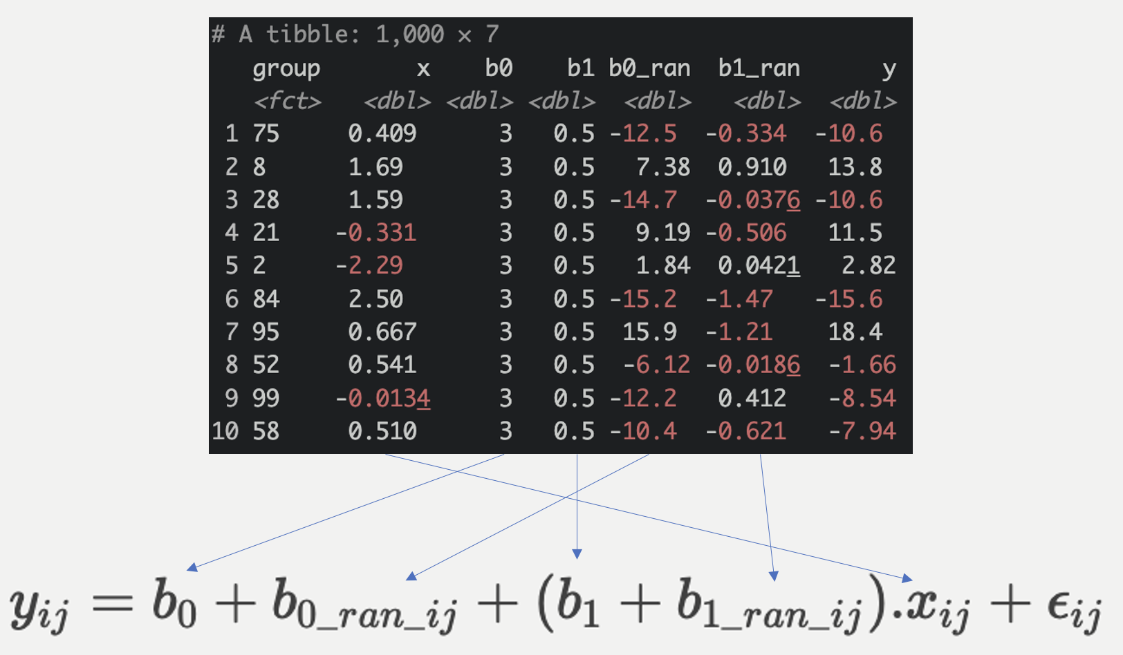
mutate(y = b0 + b0_ran + (b1 + b1_ran) * x + rnorm(n),
group = as.factor(group))
Linear Regression Model
\begin{gather} y_i = b_0 + b_1 . x_i + \epsilon_i \end{gather}
Linear Mixed Effect Model
\begin{gather} y_{ij}=b_0 + b_{0\_ran\_ij} + (b_1 + b_{1\_ran\_ij}).x_{ij} + \epsilon_{ij} \\ b_{0\_ran\_ij} \sim \text{normal}(0,10) \\ b_{1\_ran\_ij} \sim \text{normal}(0,1) \end{gather}
Did you notice the difference between the 2 models? They sure do look different! But not that different, we see b0_ran_ij and b1_ran_ij added the the equation, which we are essentially trying to simulate. Remember we said we will give each team equal amount of coffee beans upfront, then randomly add or remove them? The giving each team equal amount is b0, randomly add or remove is b0_ran_ij, where i is the ith row of data and j is the jth group (out of 100). This is our random intercept for each group.
Similarly, we stated that some groups benefit from having more coffee but some don’t. This is our random slope, which is essentially b1_ran_ij. The actual inter-group slope is the sum of average slope and random slope aka (b1 + b1_ran_ij).
Visualize Data Via Group
df |>
  ggplot(aes(x=x,y=y)) +
  geom_point() +
  geom_smooth(method = "lm") +
  facet_wrap(.~group)
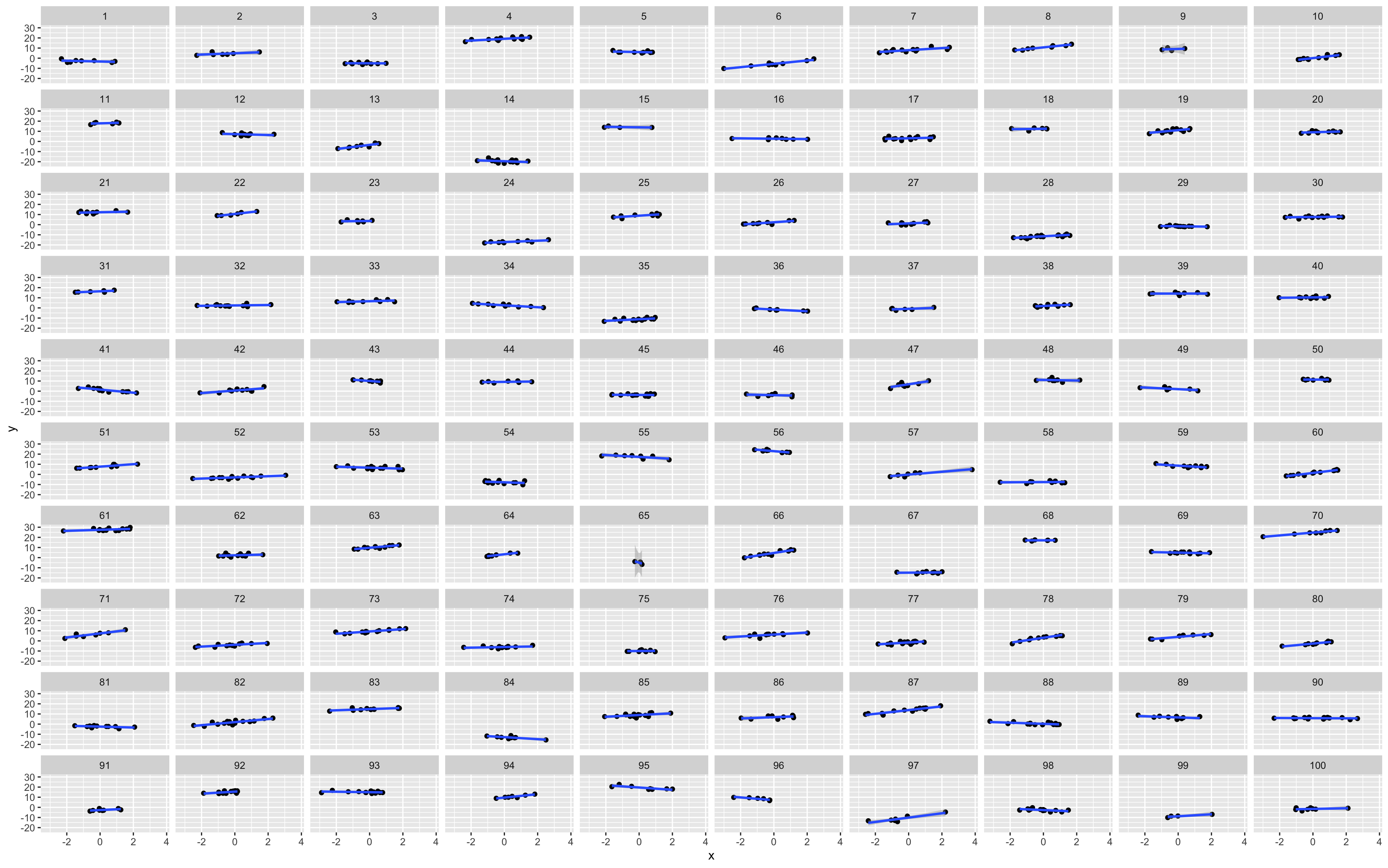
As we can see, not all groups have the same intercepts or slopes! Is it fair to lump them all up and analyze or does mixed effect modelling make more sense here? Let’s check both out!
Simple Linear Regression - Does it Make Sense?
model <- lm(y~x,df)
summary(model)
##
## Call:
## lm(formula = y ~ x, data = df)
##
## Residuals:
##     Min      1Q  Median      3Q     Max
## -25.303  -5.756   0.145   5.813  25.277
##
## Coefficients:
##             Estimate Std. Error t value Pr(>|t|)
## (Intercept)   3.6933     0.2896  12.753   <2e-16 ***
## x             0.5223     0.2759   1.893   0.0586 .
## ---
## Signif. codes:  0 '***' 0.001 '**' 0.01 '*' 0.05 '.' 0.1 ' ' 1
##
## Residual standard error: 9.153 on 998 degrees of freedom
## Multiple R-squared:  0.003579,	Adjusted R-squared:  0.00258
## F-statistic: 3.584 on 1 and 998 DF,  p-value: 0.05862
df |>
  ggplot(aes(x=x,y=y)) +
  geom_point() +
  geom_smooth(method = "lm")
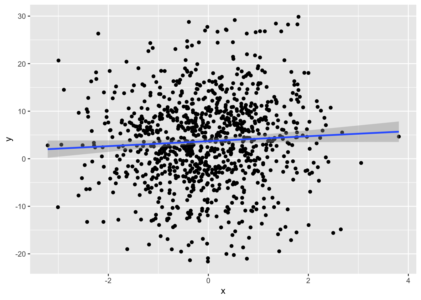
Even though the intercept and coefficient is quite close to our simulated base intercept and slope, can we really combine all data points and treating them all as independent? A few things to look at here is the std err of the estimates, and Adjusted R2, only 0.2% of variance were explained by our simple model.
Mixed Effect Modelling Via lme4
model_m <- lmer(y ~ x + (x|group), df)

summary(model_m)
## Linear mixed model fit by REML ['lmerMod']
## Formula: y ~ x + (x | group)
##    Data: df
##
## REML criterion at convergence: 3675.3
##
## Scaled residuals:
##      Min       1Q   Median       3Q      Max
## -3.00624 -0.55827 -0.00145  0.59007  2.91870
##
## Random effects:
##  Groups   Name        Variance Std.Dev. Corr
##  group    (Intercept) 81.4530  9.025
##           x            0.8011  0.895    0.00
##  Residual              0.9624  0.981
## Number of obs: 1000, groups:  group, 100
##
## Fixed effects:
##             Estimate Std. Error t value
## (Intercept)  4.11141    0.90321   4.552
## x            0.46835    0.09713   4.822
##
## Correlation of Fixed Effects:
##   (Intr)
## x 0.002
Let’s unpack! The equation y ~ x + (x|group) essentially means, we want the mixed effect model to including a random intercept for each group (1|group) and also a random slope for x (x | group), and include fixed effect of x x + (x|group). There are 2 areas here we are interested in.
Random Effects:
We are interested to see how much variance are explained by our mixed effect model. To calculate this, we essentially add all accounted variance and divided by the sum of all accounted and residual variance.
\begin{gather} \text{explained variance} = \frac{\text{Accounted variance}}{\text{Accounted variance} + \text{residual variance}} \end{gather}
which is (81.4530+0.8011) / (81.4530+0.8011+0.9624) = 0.988435 . Woo hoo! 👍 98% of the variance were explained by our mixed effect model!
Did you also notice that our random effect sd is very similar to the sd we simulated? We simulated random intercept as rnorm(0,10), the esimated sd is 9.025. Same with our random slope, we simulated it as rnorm(0,1) and estimated as 0.895.
Fixed Effects:
Our fixed effect estimates are also quite close to our simulated ones! But notice how much more certain this estimate is with std err of 0.09 and higher t value, compared to our simple linear regression model? 😎 I think we got the right model here!
Let’s Look At Random Effect Coefficients
ranef(model_m)$group |> head(10)
##    (Intercept)          x
## 1   -7.2738015 -0.7389876
## 2    0.7450866  0.1577318
## 3   -9.1134650 -0.4180497
## 4   15.0061774  0.3688105
## 5    1.9454853 -0.6675333
## 6   -9.6748163  1.1202248
## 7    3.7971551  0.5211608
## 8    6.5405664  1.0871792
## 9    4.9790977 -0.0173629
## 10  -3.9500589  1.2277225
Notice that these are not the actual coefficients, these are the addition of. The equation would be coef(model_m) = fixef(model_m) + ranef(model_m). Which when we use predict, it will estimate coef result. Let’s take a look at the 1st group and see if calculation turns out right.
Coef(model_m)
coef <- coef(model_m)$group |> head(1)
coef
##   (Intercept)          x
## 1   -3.162391 -0.2706345
Fixef(model_m)
fixef <- fixef(model_m)
fixef
## (Intercept)           x
##   4.1114100   0.4683532
Ranef(model_m)
ranef <- ranef(model_m)$group |> head(1)
ranef
##   (Intercept)          x
## 1   -7.273801 -0.7389876
Coef = fixef + ranef
fixef + ranef
##   (Intercept)          x
## 1   -3.162391 -0.2706345
coef == fixef + ranef
##   (Intercept)    x
## 1        TRUE TRUE
That’s so cool! 😎 There is further discussion on this topic on StackExchange.
How do we do this on Stan?
### write stan model
stan_mixed_effect <- "
data {
  int N;
  int g; //group
  array[N] real x;
  array[N] real y;
  array[N] int group;
}

parameters {
  real b0;
  real b1;
  array[g] real b0_ran;
  real<lower=0> b0_ran_sigma;
  array[g] real b1_ran;
  real<lower=0> b1_ran_sigma;
  real<lower=0> sigma;
}

model {
  //prior
  b0_ran ~ normal(0,b0_ran_sigma);
  b0_ran_sigma ~ uniform(0,100);
  b1_ran ~ normal(0,b1_ran_sigma);
  b1_ran_sigma ~ uniform(0,100);

  //likelihood
  for (i in 1:N) {
    for (j in 1:g) {
      if (group[i]==j) {
        y[i] ~ normal(b0 + b0_ran[j] + (b1 + b1_ran[j]) * x[i], sigma);
      }
    }
  }
}
"

mod <- cmdstan_model(write_stan_file(stan_mixed_effect))

df_stan <- list(N=n,g=group,x=x,y=df$y,group=df$group)

fit <- mod$sample(data=df_stan, seed = 123, chains = 4, parallel_chains = 4, iter_warmup = 1000, iter_sampling = 2000)

stan_sum <- fit$summary()

stan_sum
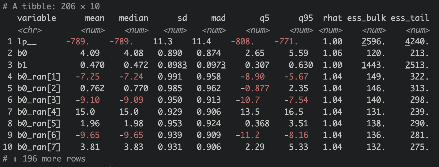
Alright, we’ve learnt that first we need to check our diagnostis for Stan model. Rhat close to 1 and < 1.05, check ✅! ESS >100, check ✅! OK, we can be comfortable with our model estimates. Notice b0 and b1 are also quite close to our set coefficients? Let’s see if both the random intercept and slope sigma estimates are similar to our set value.
Sigma’s of B0_ran and B1_ran
stan_sum |>
  filter(str_detect(variable,"b.*sigma"))
## # A tibble: 2 × 10
##   variable      mean median     sd    mad    q5   q95  rhat ess_bulk ess_tail
##   <chr>        <num>  <num>  <num>  <num> <num> <num> <num>    <num>    <num>
## 1 b0_ran_sigma 9.14   9.10  0.669  0.665  8.12  10.3   1.00    9502.    5644.
## 2 b1_ran_sigma 0.908  0.904 0.0761 0.0750 0.790  1.04  1.00    7502.    6336.
Not bad! Very similar indeed! Let’s see if the random effect is similar to lme4.
Differences of our random intercepts and slopes
## # A tibble: 100 × 7
##    group b0_ran  b1_ran `(Intercept)`       x b0_diff   b1_diff
##    <chr>  <dbl>   <dbl>         <dbl>   <dbl>   <dbl>     <dbl>
##  1 1     -7.25  -0.743         -7.27  -0.739  -0.0205  0.00450
##  2 2      0.762  0.152          0.745  0.158  -0.0169  0.00537
##  3 3     -9.10  -0.426         -9.11  -0.418  -0.0185  0.00766
##  4 4     15.0    0.367         15.0    0.369  -0.0177  0.00193
##  5 5      1.96  -0.671          1.95  -0.668  -0.0189  0.00396
##  6 6     -9.65   1.12          -9.67   1.12   -0.0212  0.00184
##  7 7      3.81   0.520          3.80   0.521  -0.0163  0.00104
##  8 8      6.56   1.09           6.54   1.09   -0.0213 -0.00109
##  9 9      5.01  -0.0187         4.98  -0.0174 -0.0287  0.00136
## 10 10    -3.93   1.23          -3.95   1.23   -0.0187  0.000527
## # ℹ 90 more rows
Not too shabby at all! Look at b0_diff and b1_diff, essentiall we’re using subtracting ranef(model_m) from stan’s b0_ran and b1_ran. Very very small differences! Awesomeness!

This is amazing! The fixed, random intercepts and slopes coefficient and their standard errors are so similar between lme4 and cmdstanr! Very reassuring!
Conclusion, given this simulated and made up dataset, for every increase in 1 unit of coffee (note we didn’t specify unit on purpose 🤣), there is a ~0.5 increase in coffee cupping score, taking into account of all 100 groups of contestants! Practice makes progress! 🙌
Acknowledgement
Thanks again to Alec Wong 👍 for correcting my Stan model. Initially I didn’t use uniform distribution for sigma of the random effect distributions and the Stan Model was very finicky and Rhat, ESS were off. But after writing the correct formula the model worked smoothly!
Lessons Learnt
- In
blogdownwe can use## Title {#title}as kind of like a slug to link url to header - coef = fixef + ranef
- learnt how to write a simple mixed effect model in
cmdstanr - learnt that we need to include parameters for estimating sigma of the random effects.
- fitting stan with mixed effect model is quite intuitive! Even though the code looked like it’s doing complete pooling.
If you like this article:
- please feel free to send me a comment or visit my other blogs
- please feel free to follow me on twitter, GitHub or Mastodon
- if you would like collaborate please feel free to contact me
- Posted on:
- October 5, 2023
- Length:
- 11 minute read, 2165 words
- Categories:
- r R stan cmdstanr bayesian beginner mixed effect model hierarchical model