An Educational Stroll With Stan - Part 3

Diving into this, we’re exploring how using numbers to express our certainty, especially with medical results, can help sharpen our estimated ‘posterior value’ and offer a solid base for learning and discussions. We often talk about specifics like sensitivity without the nitty-gritty math, but crafting our own priors and using a dash of Bayes and visuals can really spotlight how our initial guesses shift. Sure, learning this takes patience, but once it clicks, it’s a game-changer – continuous learning for the win!

Previously, we familiarized ourselves to simple linear and logistic regression models using cmdstanr. Today, we’re going to explore a bit more practicality of bayes’ theorem in clinical setting.

Disclaimer:

This is not medical advice, nor is it a definitive method for application. This tool, like any other, is utilized to understand the prior, likelihood, and posterior. Everything conducted here is simulated, utilizing assumed sensitivity and specificity values, which can be derived from medical literature.

Prior Is Not As Easy As We Think

Quantifying clinical intuition or judgment is no easy task. Our minds typically gravitate towards binary outcomes: it either is, or it is not. Unfortunately, Bayes’ Theorem does not operate in this manner. It necessitates a distribution and the probability of a condition. When we suspect or NOT suspect a clinical condition, we should strive to estimate it with a range and distribution, for example, a condition is about 50% with an sd of ~20%. This will give a range of possible values

A Quick Recap of Bayes’ Theorem

\begin{equation} p(\text{disease+}|\text{test+}) = \frac{p(\text{test+}|\text{disease+}) \cdot p(\text{disease+})}{p(\text{test+})} \end{equation}

The equation above is positive predictive value, meaning what is the probability of having a condition given a test positive. p(disease+) is essentially our prior, our clinical gestalt (perhaps from history, physical exam, certain data).

Today, we’ll attempt to explore this clinical applicability and open our eyes to probability theory.

Objectives

• Load Library & Simulate Sensitivity / Specificity Data
• Stan Model For Estimating Sens/Spec
• Clinical Prior Using Beta-Binomial Distribution
• Write Our PPV/NPV formula in Stan
  • Extract our PPVs
  • Visualize Our PPV with Prior
  • Extract our NPV & Visualize
• Let’s Look At Multiple Priors
• Acknowledgement
• Final Thought
• Lessons Learnt

Load Library & Simulate Sensitivity / Specificity Data

Let’s assume that we have a set of data set that we can estimate the sensitivity and specificity of a test. Let’s hypothetically call this test prokalcitony 🤣. Given a hypothetical medical literature, the estimated sensitivity is 98% (95%CI 95-100) and specificity of 90% (95%CI 85-92) if threshold is set at < 0.05.

library(tidyverse)
library(cmdstanr)
library(bayesplot)

# assuming prokalcitony has sens of 98% (95%CI 95-100) and spec of 90% (95%CI 85-92)
sens_spec_calc <- function(point,ci,num) {
  point_ci_diff <- abs(point-ci)
  std <- point_ci_diff/1.96
  mu <- point
  var <- std^2
  alpha <- ((1 - mu) / var - 1 / mu) * mu ^ 2
  beta <- alpha * (1 / mu - 1)
  return_vector <- rbeta(num,alpha,beta)
  return(return_vector)
}

#simulated data, assuming we have data to run thru stan and mcmc
n <- 1000
set.seed(1)
pos_disease <- rbinom(n/2,1,sens_spec_calc(point=0.98,ci=0.95, num=n)) 
neg_disease <- rbinom(n/2,1,sens_spec_calc(point=0.9,ci = 0.85,num=n)) 
neg_disease <- ifelse(neg_disease==1,0,1)


df <- list(N=n, disease=c(rep(1,n/2),rep(0,n/2)), test=c(pos_disease,neg_disease))

Let’s explore the code above. The function of sens_spec_calc essentially creates a beta-binomial distribution just so we’re not tied to one point estimate, but rather a distribution. Hypothetically, let’s say we do have this dataset (simulated), we can then estimate the sensitivity and specificity. Then use it to assess how our prior changes given a test result.

Stan Model For Estimating Sens/Spec

#stan model for estimating sens and spec of simulated data
diagnostic_stan <- '
data {
  int N;
  array[N] int test;
  array[N] int disease;
}

parameters {
  real<lower=0,upper=1> sensitivity;
  real<lower=0,upper=1> specificity;
}

model {
  //prior
  sensitivity ~ uniform(0,100);
  specificity ~ uniform(0,100);

  
  // Likelihood
  for (i in 1:N) {
    if (disease[i] == 1) {
      test[i] ~ bernoulli(sensitivity);
    } else {
      test[i] ~ bernoulli(1-specificity);
    }
  }
  
}
'

# running it without stan file
mod <- cmdstan_model(write_stan_file(diagnostic_stan))

fit <- mod$sample(data=df, seed = 123, chains = 4, parallel_chains = 4, iter_warmup = 1000, iter_sampling = 2000, show_messages = F)

#fit$summary()

#mcmc_trace(fit$draws())

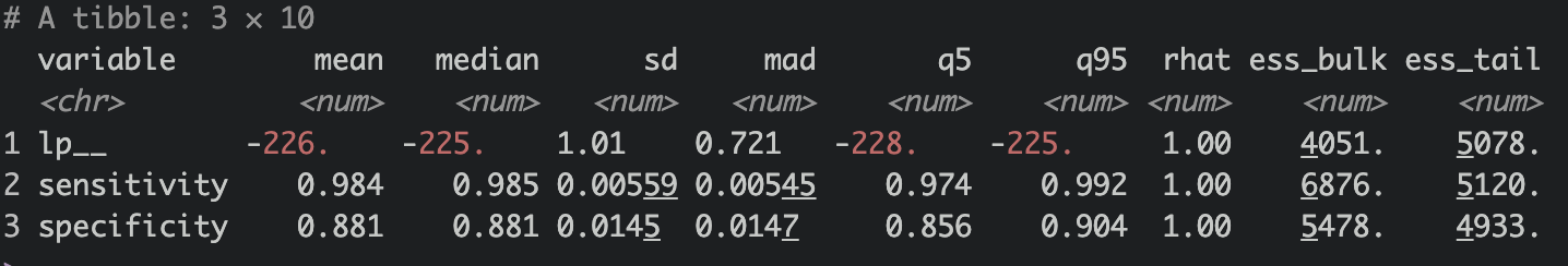
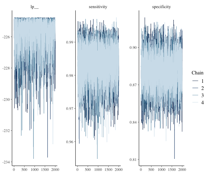
Nice! The sen and spec estimates and its 95% CI are very similar to how we set them. Let’s extract the sens and spec chains and use them to our advantage to estimate our ppv / npv.

# extracting all sens of all 4 chains (excluding warm up)
sens <- fit$draws(variables = "sensitivity") |> 
  as.data.frame() |>
  unlist()

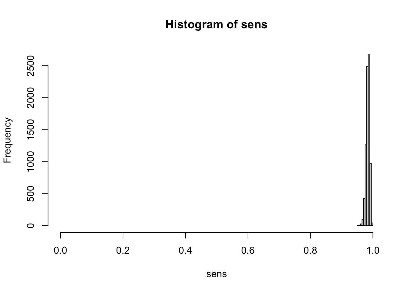
hist(sens, xlim=c(0,1))

# extracting all spec of all 4 chains (excluding warm up)
spec <- fit$draws(variables = "specificity") |>
  as.data.frame() |> 
  unlist()

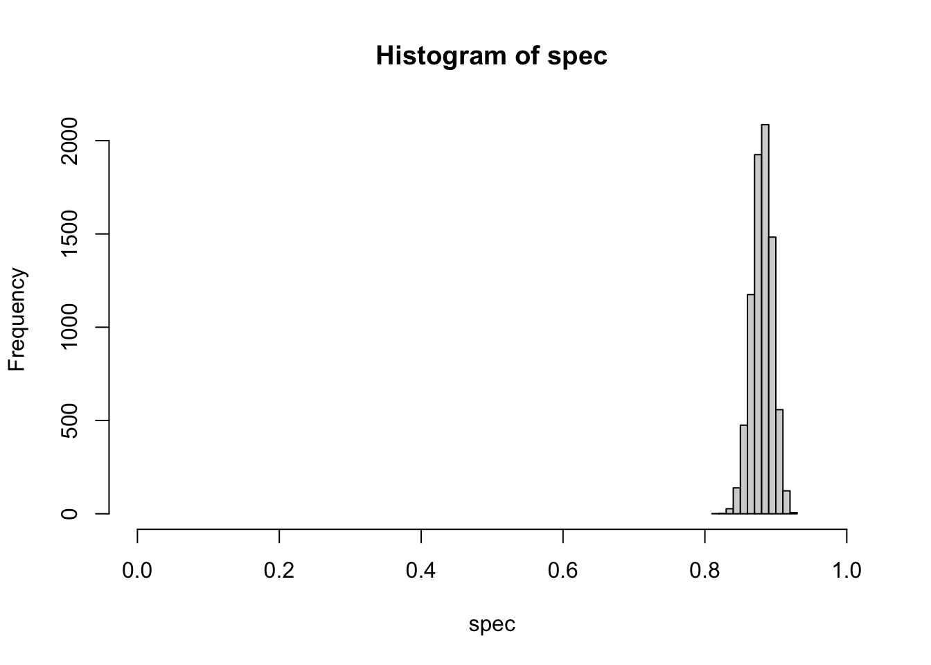
hist(spec, xlim=c(0,1))

Clinical Prior Using Beta-Binomial Distribution

# write a function to set our clinical prior using beta-binomial
prior_beta <- function(mu,std) { 
  var <- std^2
  alpha <- ((1 - mu) / var - 1 / mu) * mu ^ 2
  beta <- alpha * (1 / mu - 1)
  return(list(alpha=alpha,beta=beta))
}

# assuming we have 30% suspicion that the person has disease with an sd of 10%
pb <- prior_beta(0.3,0.1)
prior <- rbeta(length(sens),shape1 = pb$alpha, shape2 = pb$beta)
hist(prior, xlim=c(0,1))

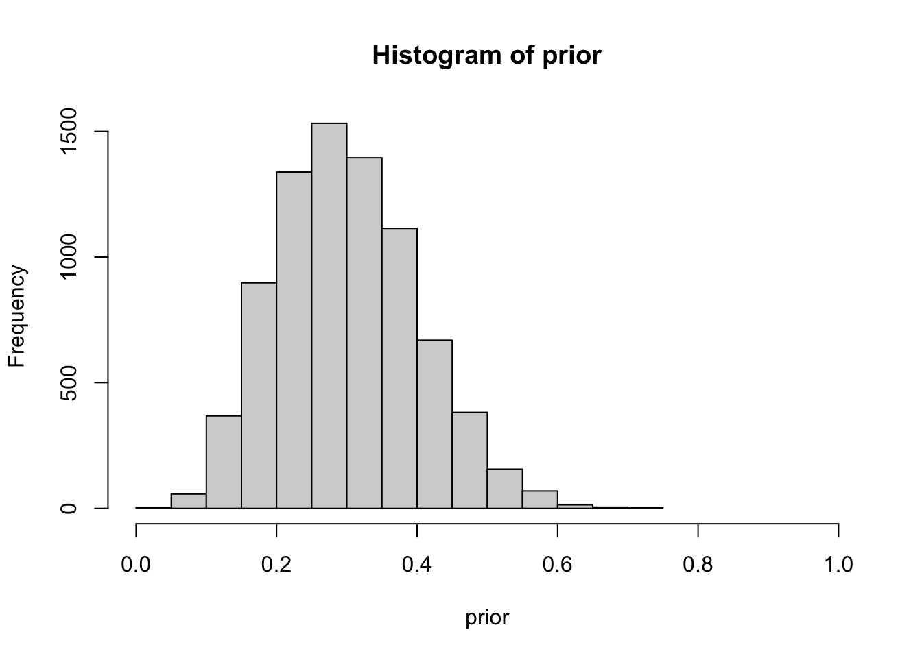
Quantifying our prior, as previously discussed, poses a significant challenge. The difficulty arises in translating a binary thought process into a distribution. Within epidemiology, we encounter metrics like incidence and prevalence, which are essentially point estimates, thereby facilitating the assignment of a number to our prior more straightforwardly. Cultivating the skill to quantify uncertainty necessitates practice and a comfort with embracing ranges and unpredictability. Several distributions are available to assist in this, such as the familiar binomial distribution, and others that offer more flexibility like the beta-binomial distribution. The latter provides alpha and beta parameters which assist in shaping the desired distribution, as demonstrated in the previous example. To simplify matters, we can devise a function that utilizes mean and sd to convert alpha and beta for us.

In the above example, we simulated a beta-binomial distribution with a mean of 30% and a standard deviation of 10%. You can essentially experiment with these values to practice shaping the ranges of your clinical gestalt or prior. Observe that the range is bounded between 0 and 1. Additionally, the distribution appears to be wider than the sensitivity and specificity in previous plots. We are essentially asserting that we suspect there is a mean 30% probability of the patient having the disease, with a standard deviation of 10%, ranging from 0 to 60%. This also indicates that, while we are not entirely certain, we harbor less suspicion that the patient has the disease. The threshold is arbitrary, but we’ll set >55% as a benchmark

Write Our PPV/NPV formula in Stan

#diag pred model
diag_pred <- "
data {
  int N;
  array[N] real sens;
  array[N] real spec;
  array[N] real prior;
}

generated quantities {
  array[N] real ppv;
  array[N] real npv;
  
  for (i in 1:N) {
    ppv[i] = sens[i]*prior[i] / ((sens[i]*prior[i])+((1-prior[i])*(1-spec[i])));
    npv[i] = ((1-prior[i])*spec[i]) / (((1-prior[i])*spec[i])+(prior[i]*(1-sens[i])));
  }
}
"

mod2 <- cmdstan_model(write_stan_file(diag_pred))

# set our clinical prior
df_prior <- list(N=length(sens),sens=sens,spec=spec,prior=prior)

# fit fixed_param
fit2 <- mod2$sample(data = df_prior, chains = 1, iter_sampling = 1, fixed_param = T, show_messages=F)

# extract all ppv and npv
df_param <- as.data.frame(fit2$summary()) 

Let’s break down what the code means. To calculate the positive predictive value (aka p(disease+|test+)) (refer to the formula at the beginning of the blog), we need to examine p(test+|disease+), also known as sensitivity, multiplied by the prior, and then divide by p(test+), or the total positive test results. This latter is calculated as [sensitivity * prior + (1-specificity) * (1-prior)].

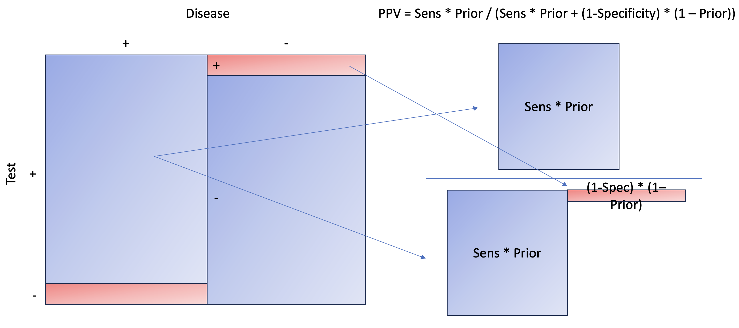We essentially aim to calculate the areas to the right, marginalizing on the positive test, which can also be interpreted as the probability of a disease given a positive test. To calculate the area, you need to multiply the length and width. Here, our length is sensitivity and 1 − specificity, while our width is prior and 1 − prior.

Let’s take a look at Negative Predictive Value, aka probability of NOT having disease given test negative. 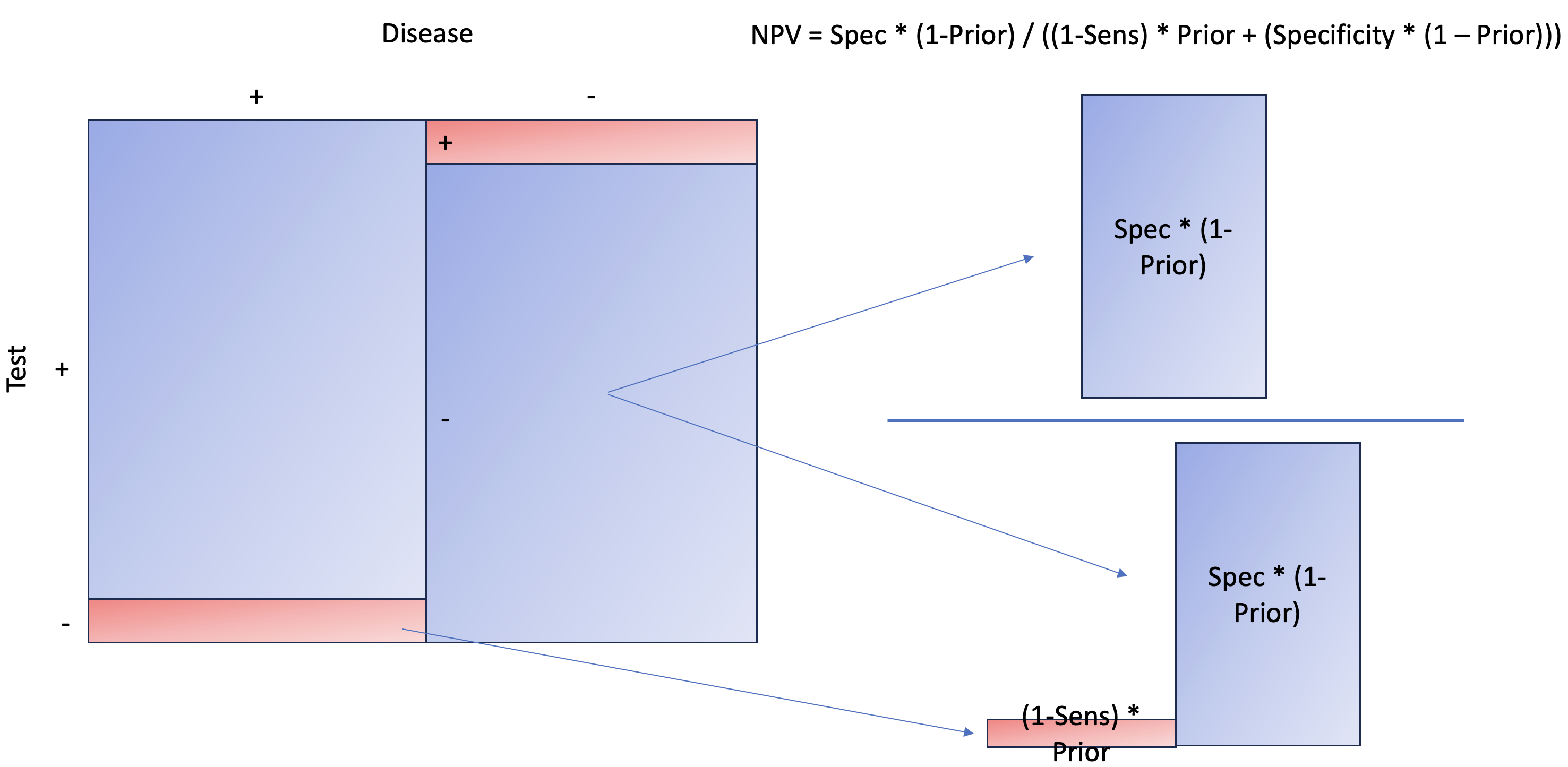As you can see, the concept is the same as PPV, except we are now interested in the NOT disease state when the test is negative. Later, at the end of the article, you’ll see that it makes more sense to estimate the probability of disease given a negative result. This is not only more intuitive but also more relatable than NPV itself.

Let’s take a look at our first 10 summary of generated quantities.

df_param |> head(10)

##    variable     mean   median sd mad       q5      q95 rhat ess_bulk ess_tail
## 1    ppv[1] 0.761350 0.761350 NA   0 0.761350 0.761350   NA       NA       NA
## 2    ppv[2] 0.717160 0.717160 NA   0 0.717160 0.717160   NA       NA       NA
## 3    ppv[3] 0.810141 0.810141 NA   0 0.810141 0.810141   NA       NA       NA
## 4    ppv[4] 0.631920 0.631920 NA   0 0.631920 0.631920   NA       NA       NA
## 5    ppv[5] 0.791641 0.791641 NA   0 0.791641 0.791641   NA       NA       NA
## 6    ppv[6] 0.792706 0.792706 NA   0 0.792706 0.792706   NA       NA       NA
## 7    ppv[7] 0.868056 0.868056 NA   0 0.868056 0.868056   NA       NA       NA
## 8    ppv[8] 0.745761 0.745761 NA   0 0.745761 0.745761   NA       NA       NA
## 9    ppv[9] 0.742902 0.742902 NA   0 0.742902 0.742902   NA       NA       NA
## 10  ppv[10] 0.798960 0.798960 NA   0 0.798960 0.798960   NA       NA       NA

Notice how our mean, median, 5%, and 95% all have the same value? That is because every row (e.g., PPV[1], PPV[2]) is an exact calculation of PPV using the distribution of sensitivity (sens), specificity (spec), and prior. Since each row will have different sens, spec, and prior values, given their distribution, we will have a different PPV. Essentially, we have over 8000 PPVs, from which we can construct a distribution. The same applies to NPV.

Extract our PPVs

ppv <- df_param |>
  filter(str_detect(variable,"ppv")) |>
  pull(mean)

Write A Visualization Function

# visualize transformation of ppv and prior, write a function
visualize <- function(pred_val, label1, label2, ps=NULL) {
df <- tibble(pred={{pred_val}},prior=prior) 

# max density to label prior and value for info
vec_pred <- pred_val |> density() 
vec_pred <- vec_pred$y |> max()
vec_prior <- prior |> density() 
vec_prior <- vec_prior$y |> max()

max_vec <- max(vec_pred,vec_prior)

add <- case_when(
  max_vec>=15 & max_vec <20 ~1.5,
  max_vec>20 & max_vec < 50 ~ 3,
  max_vec>=50 & max_vec < 100 ~ 4,
  max_vec>=100 & max_vec < 300 ~10,
  max_vec>=300 ~30,
  TRUE ~ 0.5)


graph <- 
  ggplot() +
  geom_density(data=df, mapping = aes(x=pred), color = "blue", fill = "blue", alpha = 0.5) +
  geom_density(data=df, mapping = aes(x=prior), color = "red", fill = "red", alpha = 0.5) +
  annotate(x=0.5,y=max_vec+add, geom = "text", label=paste0("Prior Median: ", df$prior |> median() |> round(digits = 2), " (95% CI ", quantile(df$prior, 0.025) |> round(digits = 2), "-", quantile(df$prior, 0.975) |> round(digits = 2),")")) +
  annotate(x=0.5,y=max_vec, geom = "text", label=paste0(label1, " Median: ", df$pred |> median() |> round(digits = 2), " (95% CI ", quantile(df$pred, 0.025) |> round(digits = 2), "-", quantile(df$pred, 0.975) |> round(digits = 2),")")) +
  ggtitle(label = paste0(label2," Predictive Value (blue), Prior ", ps ," (red)")) +
  theme_minimal()

return(graph)
  
}

Visualize Our PPV with Prior

#visualize ppv
visualize(ppv, "PPV", "Positive")

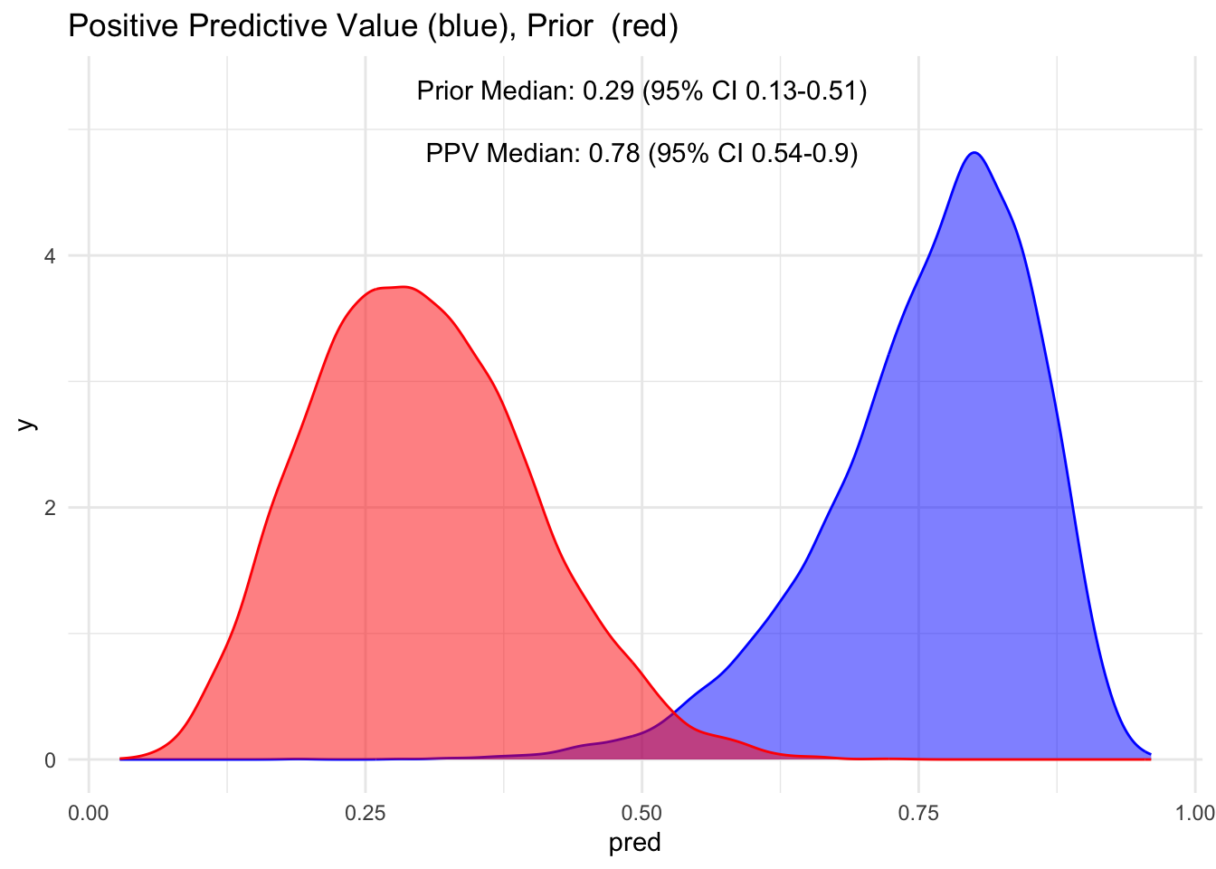
Notice how the red distribution shifts to blue when the test is positive? We had a median prior of 30%, which shifts to 78% when the test is positive. This is quite an increase. However, also observe that the 95% credible interval ranges from 54-90%, meaning we’re not entirely certain if a person has the disease, even given a positive test.

What if our test is negative? What does it say about the probability of having the disease?

Extract our NPV

npv <- df_param |>
  filter(str_detect(variable,"npv")) |>
  pull(mean)

# we want to know what percentage is with disease
npv <- 1- npv

# visualize 1-npv
visualize(npv, "1-NPV", "1 - Negative")

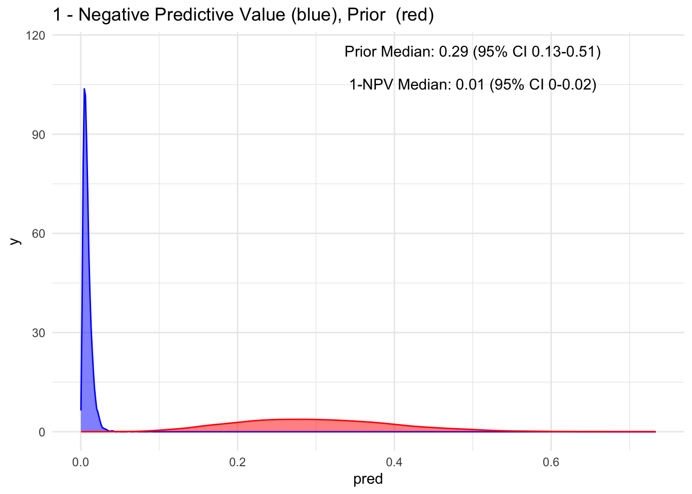
Wow, observe the transformation from red to blue when a test is negative! Our posterior median drops to 1%, with a 95% credible interval spanning from 0 to 2% for having the disease. This represents a significant decrease and introduces a higher level of certainty.

As mentioned earlier, to maintain a consistent mindset, it is more logical to consider the probability of the disease even in the context of a negative test result, which is essentially 1−NPV. This perspective provides insight into the likelihood of missing a diagnosis.

Let’s Look At Multiple Priors

Given that the test’s sensitivity is quite robust, let’s examine how the posterior probability appears with various priors. For simplicity, we’ll sequence the prior from 10 to 90%, maintaining a standard deviation of 10%.

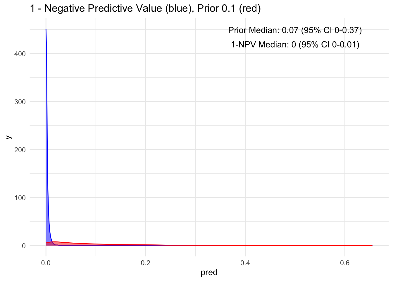
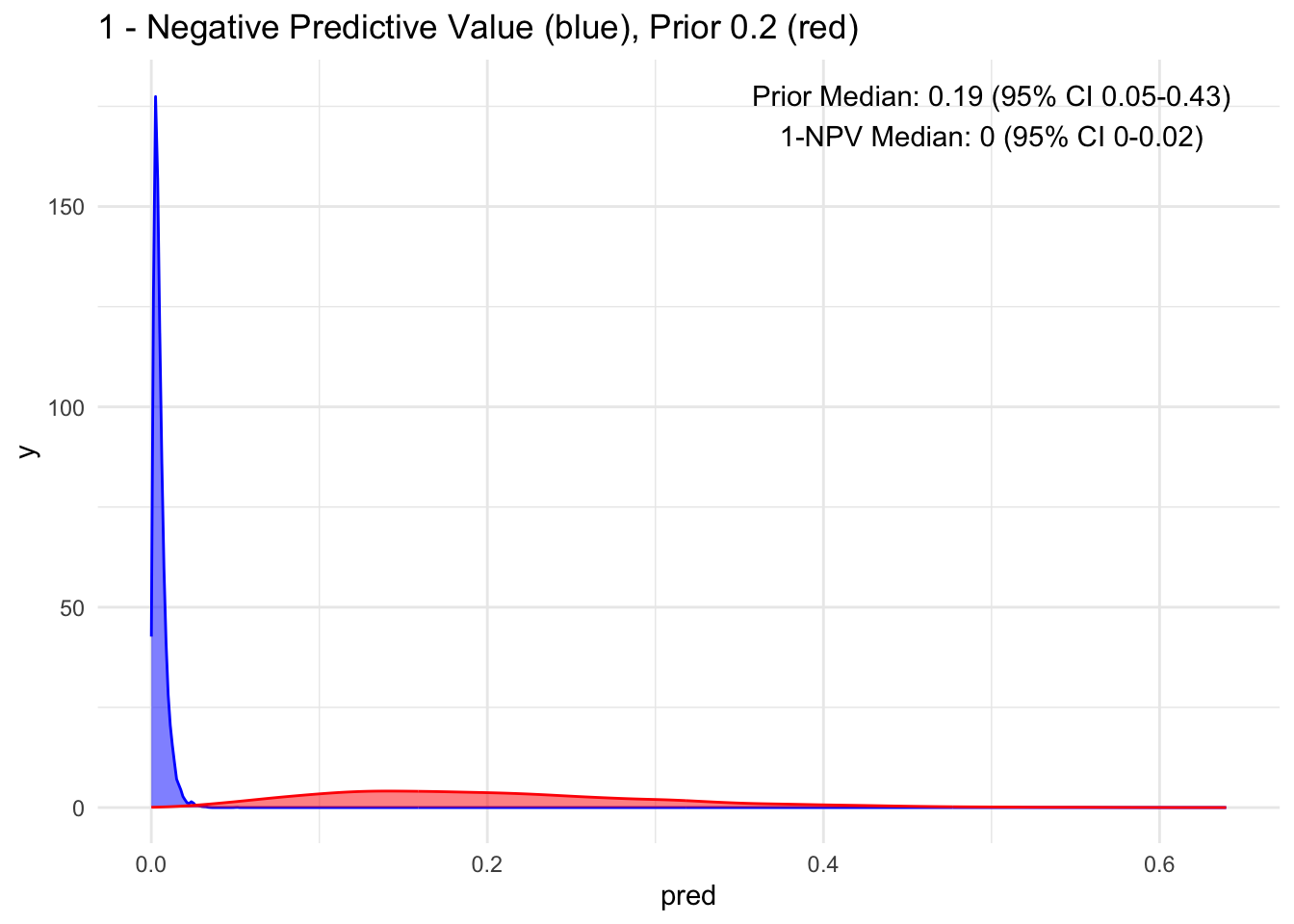
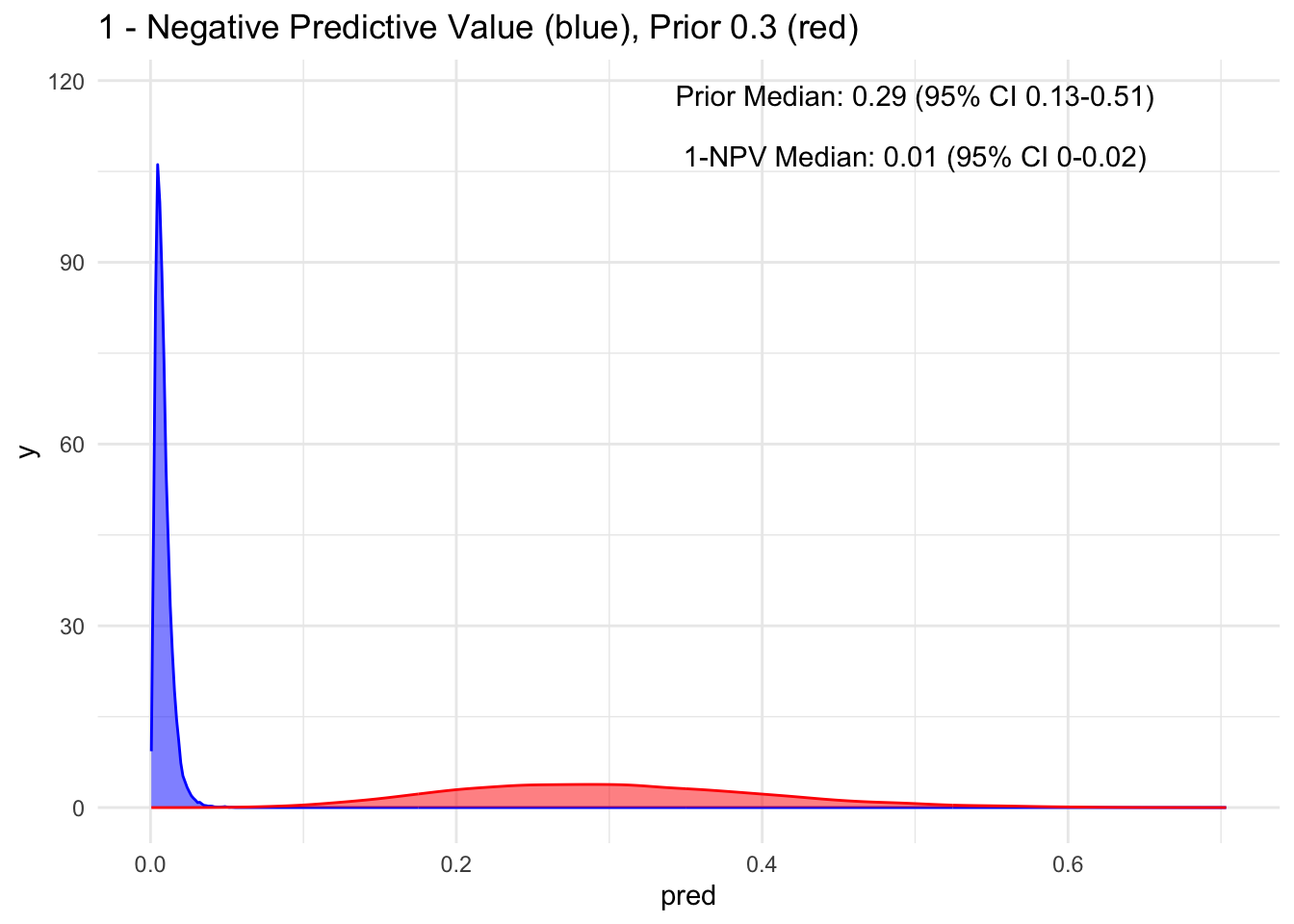
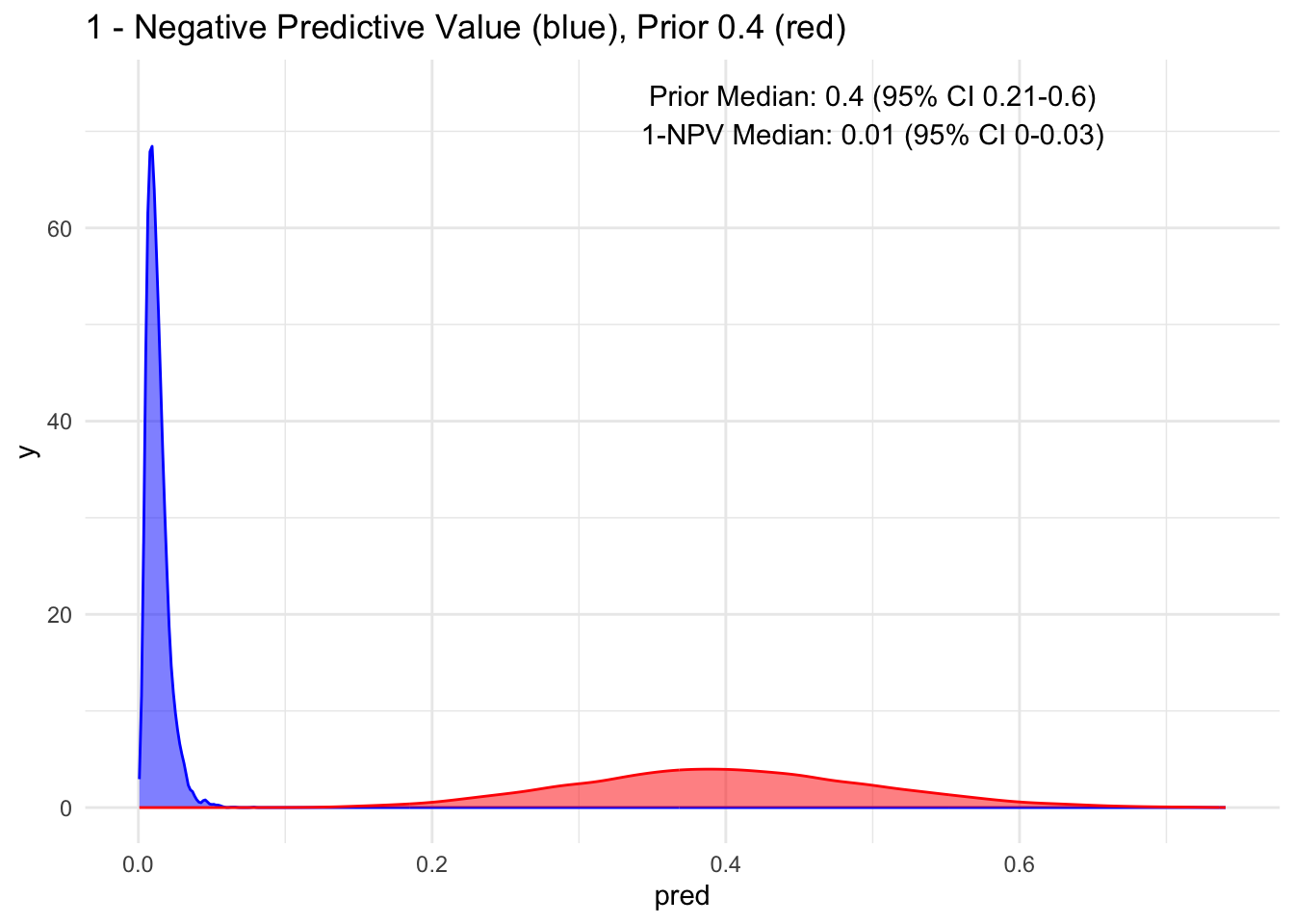
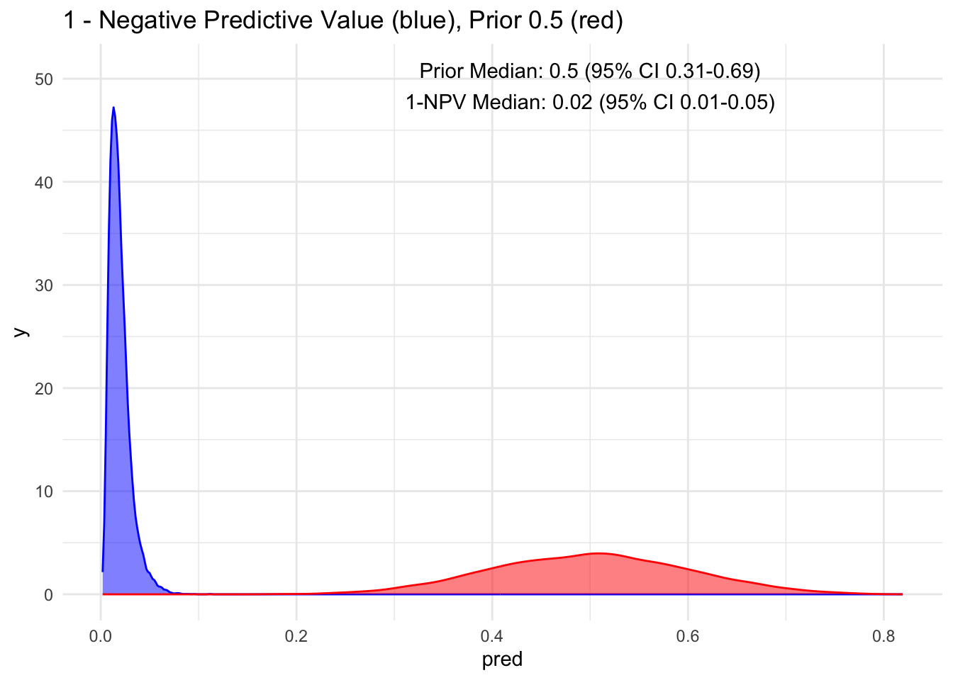
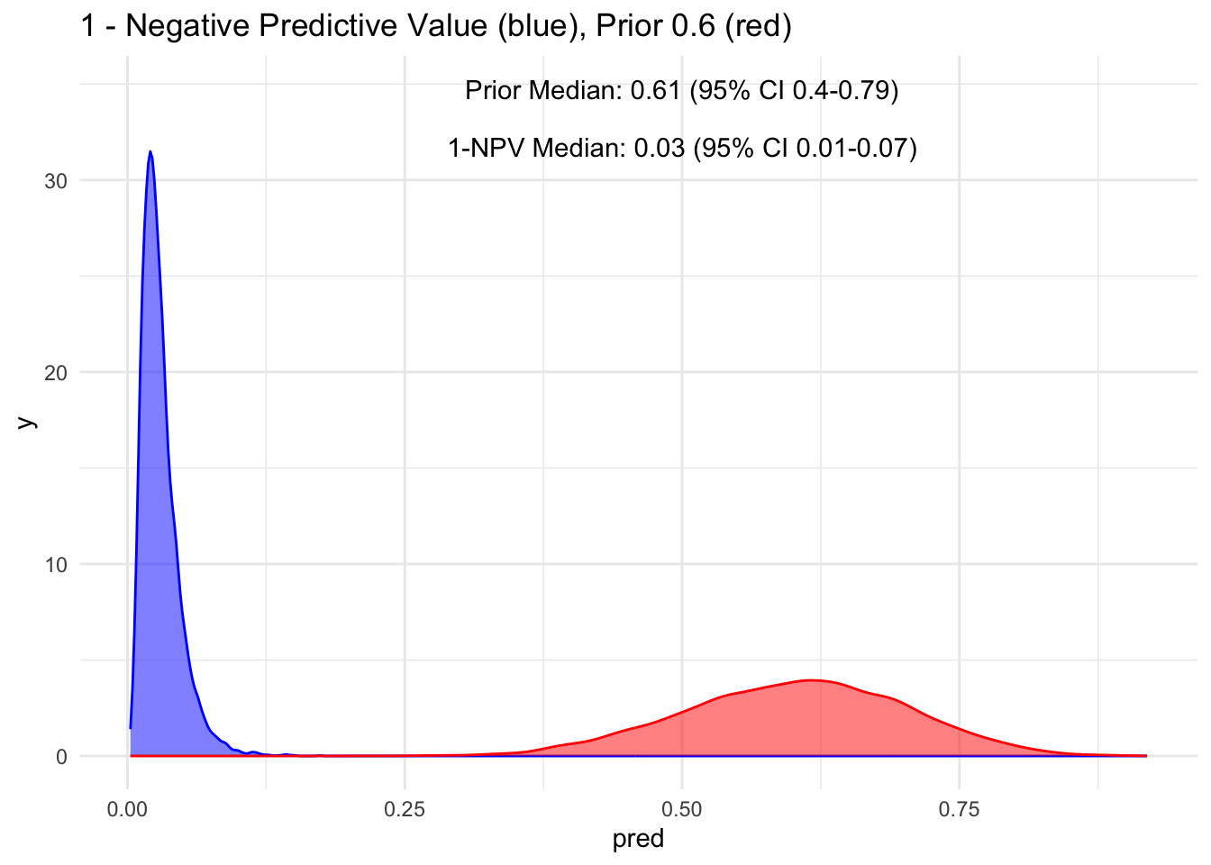
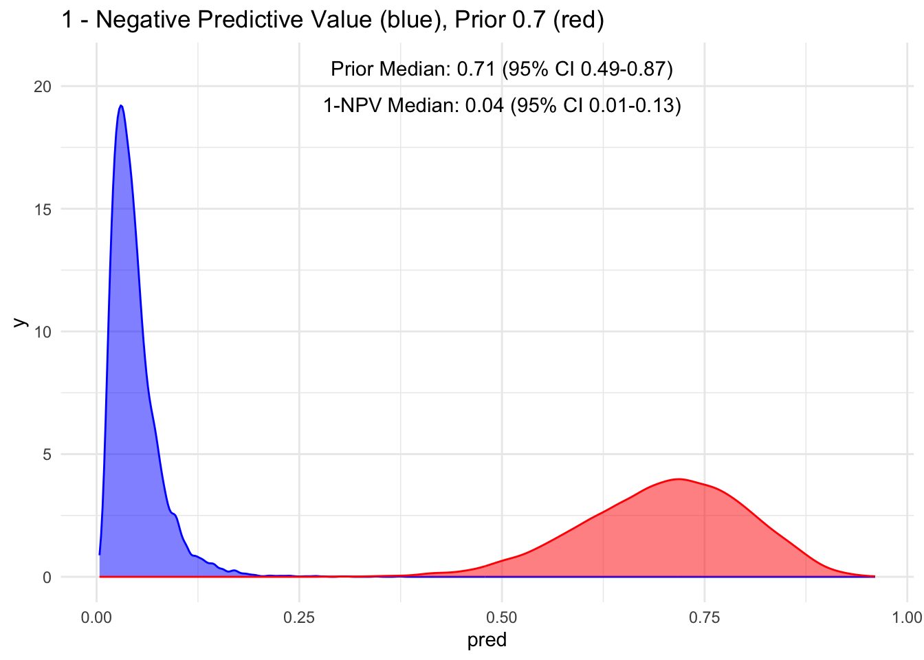
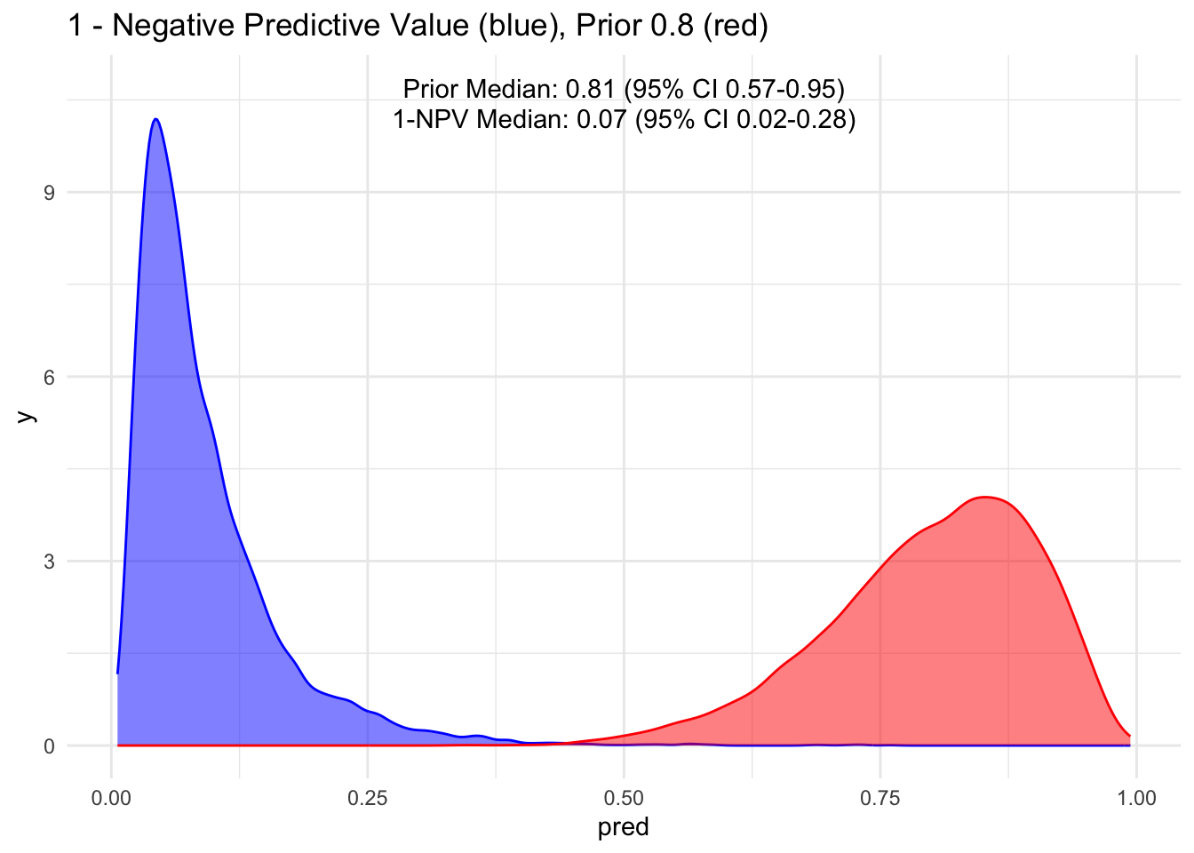
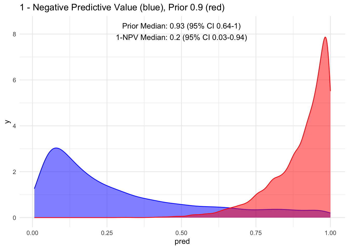
Because the sensitivity is quite high for this hypothetical test, we observe that the 95% credible interval (CI) remains relatively narrow up to a prior set at 70%. Beyond that point, we begin to see a widening of the credible intervals, even with a low median of disease process. This suggests that a negative test does not necessarily rule out the disease process if the initial degree of clinical suspicion is already high to begin with, in this case, >70%.

Additionally, it’s crucial to note that ruling out a condition does not equate to a 100% certainty of its absence; rather, it represents a probability threshold below which the disease is deemed unlikely.

Acknowledgement:

Special thanks 🙏 once again to Alec Wong, the Master of Bayes’, for enhancing my understanding of MCMC and Bayes’ Theorem. He astutely pointed out that we could consolidate both Stan codes as follows…

diagnostic_stan <- '
data {
  int N;
  array[N] int test;
  array[N] int disease;
}

parameters {
  real<lower=0,upper=1> prior_disease;
  real<lower=0,upper=1> sensitivity;
  real<lower=0,upper=1> specificity;
}

model {
  //prior
  prior_disease ~ beta(6, 14);
  sensitivity ~ uniform(0,100);
  specificity ~ uniform(0,100);

  // Likelihood
  for (i in 1:N) {
    test[i] ~ bernoulli(disease[i] * sensitivity + (1-disease[i]) * (1-specificity));
  }
}

generated quantities {
  real ppv;
  real npv;

  ppv = sensitivity*prior_disease / ((sensitivity*prior_disease)+((1-prior_disease)*(1-specificity)));
  npv = ((1-prior_disease)*specificity) / (((1-prior_disease)*specificity)+(prior_disease*(1-sensitivity)));
}
'

And it should do the exact same thing. Of course, his code looks so much more elegant than mine! 🤣

Final Thought:

The purpose of showcasing this is to illustrate that if we can quantify our certainty and uncertainty, given a test value or an exam that has sensitivity and specificity derived from medical literature, we can calculate the estimated posterior value along with its distribution. While it might be mentally overwhelming to do this for all cases and values (including history, exam, and diagnostics), speaking in numerical terms when we believe we’ve reached a certain gestalt or posterior value provides a concrete basis for discussion and learning.

While sensitivity and specificity are typically considered as fixed estimates with their respective distributions, priors and posteriors are not. Frequently, discussions about sensitivity and specificity occur without a mathematical or simulation-based understanding, as showcased here. We’ve all learned the acronyms SNout (rule out) and SPin (rule in) as quick and easy ways to remember their meanings. While having high values (~ >95%) can be helpful, dealing with moderate values may not allow us to accurately estimate our uncertainty in our heads.

Similarly, we often refer to positive predictive and negative predictive values using the prevalence directly from the studies themselves. In this demonstration, we have illustrated the flexibility of creating our own prior, attempting to quantify them, and utilizing Bayes’ theorem, visualization, and observation of the estimates and their 95% credible intervals to comprehend the magnitude of change in prior probability.

Things To Learn Next:

• Explore full-luxury bayes explored by Jose on previous post with Stan, especially with unobserved parameters. Oh it’s going to be interstingly slow… in terms of computating time
• Learn hierarchical / mixed effect modelling in Stan
• Learn about Gaussian Process in Stan

Lessons Learnt:

• We do not need separate Stan file to use cmdstan, can pass through with write_stan_file
• We can combine all Stan Code without separating them
• We don’t necessarily need Stan for the above exercise, plain old R will do.
• Probability theory is not intuitive, it is a learnt skill that requires practice, using simulation will help one understand it better

If you like this article:

• please feel free to send me a comment or visit my other blogs
• please feel free to follow me on twitter, GitHub or Mastodon
• if you would like collaborate please feel free to contact me