Testing Super Learner's Coverage - A Note To Myself
By Ken Koon Wong in r R superlearner xgboost random forest glm nnls tmle
January 2, 2026
Testing Super Learner with TMLE showed some interesting patterns 🤔 XGBoost + random forest only hit ~54% coverage, but tuned xgboost + GLM reached ~90%. Seems like pairing flexible learners with stable (even misspecified) models helps? Need to explore this more with different setups 📊

Motivations:
We have previously looked at TMLE without Super Learner and observed the poor coverage of TMLE with unspecified xgboost when compared to a correctly specified logistic regression. Now since we’ve learnt NNLS the default method behind Super Learner, why dont we test it out and take a look at the coverage! Let’s take a look at our previous coverage plot.
 We saw that with xgboost and TMLE, our coverage is about 71.1-87.6% and the lower and upper tails are asymmetrical. What if we use SuperLearner, can we improve these coverage?
Objectives
Let’s Code
We will be using the same data generating mechanism as before, but this time we will be using Super Learner to estimate the propensity score and outcome regression.Let’s write a code where we can use multicore and also a cheap 2nd hand lenovo with quad-core and Ubuntu to run and store results. Part of my learning goal for 2026 is to experiment more with parallel computing and see if we can explore mathematical platonic space more using simulation! Stay tuned on that, more to come on the simple parallel computing cluster set up!
code
library(dplyr)
library(SuperLearner)
library(future)
library(future.apply)

# Set up parallel processing
plan(multicore, workers = 4)

set.seed(1)

n <- 10000
W1 <- rnorm(n)
W2 <- rnorm(n)
W3 <- rbinom(n, 1, 0.5)
W4 <- rnorm(n)

# TRUE propensity score model
A <- rbinom(n, 1, plogis(-0.5 + 0.8*W1 + 0.5*W2^2 + 0.3*W3 - 0.4*W1*W2 + 0.2*W4))

# TRUE outcome model
Y <- rbinom(n, 1, plogis(-1 + 0.2*A + 0.6*W1 - 0.4*W2^2 + 0.5*W3 + 0.3*W1*W3 + 0.2*W4^2))

# Calculate TRUE ATE
logit_Y1 <- -1 + 0.2 + 0.6*W1 - 0.4*W2^2 + 0.5*W3 + 0.3*W1*W3 + 0.2*W4^2
logit_Y0 <- -1 + 0 + 0.6*W1 - 0.4*W2^2 + 0.5*W3 + 0.3*W1*W3 + 0.2*W4^2

Y1_true <- plogis(logit_Y1)
Y0_true <- plogis(logit_Y0)
true_ATE <- mean(Y1_true - Y0_true)

df <- tibble(W1 = W1, W2 = W2, W3 = W3, W4 = W4, A = A, Y = Y)

tune = list(
  ntrees = c(500,1000),           # More trees for better performance
  max_depth = c(3,5),                    # Deeper trees capture interactions
  shrinkage = c(0.001,0.01)    # Finer learning rate control
)

learners <- create.Learner("SL.xgboost", tune = tune, detailed_names = TRUE, name_prefix = "xgb")

# Super Learner library
SL_library <- list(c("SL.xgboost", "SL.ranger", "SL.glm", "SL.mean"),
                   c("SL.xgboost","SL.ranger"),
                   c("SL.xgboost","SL.glm"),
                   list("SL.ranger", c("SL.xgboost", "screen.glmnet")),
                   c(learners$names, "SL.glm"))

# sample
n_sample <- 1000
n_i <- 6000

# Function to run one TMLE iteration
run_tmle_iteration <- function(seed_val, df, n_i, SL_library) {
  set.seed(seed_val)
  data <- slice_sample(df, n = n_i, replace = T) |> select(Y, A, W1:W4)

  # Prepare data
  X_outcome <- data |> select(A, W1:W4) |> as.data.frame()
  X_treatment <- data |> select(W1:W4) |> as.data.frame()
  Y_vec <- data$Y
  A_vec <- data$A

  # Outcome model
  SL_outcome <- SuperLearner(
    Y = Y_vec,
    X = X_outcome,
    family = binomial(),
    SL.library = SL_library,
    cvControl = list(V = 5)
  )

  # Initial predictions
  outcome <- predict(SL_outcome, newdata = X_outcome)$pred

  # Predict under treatment A=1
  X_outcome_1 <- X_outcome |> mutate(A=1)
  outcome_1 <- predict(SL_outcome, newdata = X_outcome_1)$pred

  # Predict under treatment A=0
  X_outcome_0 <- X_outcome |> mutate(A=0)
  outcome_0 <- predict(SL_outcome, newdata = X_outcome_0)$pred

  # Bound outcome predictions to avoid qlogis issues
  outcome <- pmax(pmin(outcome, 0.9999), 0.0001)
  outcome_1 <- pmax(pmin(outcome_1, 0.9999), 0.0001)
  outcome_0 <- pmax(pmin(outcome_0, 0.9999), 0.0001)

  # Treatment model
  SL_treatment <- SuperLearner(
    Y = A_vec,
    X = X_treatment,
    family = binomial(),
    SL.library = SL_library,
    cvControl = list(V = 5)
  )

  # Propensity scores
  ps <- predict(SL_treatment, newdata = X_treatment)$pred

  # Truncate propensity scores
  ps_final <- pmax(pmin(ps, 0.95), 0.05)

  # Calculate clever covariates
  a_1 <- 1/ps_final
  a_0 <- -1/(1 - ps_final)
  clever_covariate <- ifelse(A_vec == 1, 1/ps_final, -1/(1 - ps_final))

  epsilon_model <- glm(Y_vec ~ -1 + offset(qlogis(outcome)) + clever_covariate,
                       family = "binomial")
  epsilon <- coef(epsilon_model)

  updated_outcome_1 <- plogis(qlogis(outcome_1) + epsilon * a_1)
  updated_outcome_0 <- plogis(qlogis(outcome_0) + epsilon * a_0)

  # Calc ATE
  ate <- mean(updated_outcome_1 - updated_outcome_0)

  # Calc SE
  updated_outcome <- ifelse(A_vec == 1, updated_outcome_1, updated_outcome_0)
  se <- sqrt(var((Y_vec - updated_outcome) * clever_covariate +
                   updated_outcome_1 - updated_outcome_0 - ate) / n_i)

  return(list(ate = ate, se = se))
}

# Run iterations in parallel
for (num in 1:length(SL_library)) {
cat("TMLE iterations in parallel with 4 workers (multicore)...\n")
start_time <- Sys.time()

results_list <- future_lapply(1:n_sample, function(i) {
  result <- run_tmle_iteration(i, df, n_i, SL_library[[num]])
  if (i %% 100 == 0) cat("Completed iteration:", i, "\n")
  return(result)
}, future.seed = TRUE)

end_time <- Sys.time()
run_time <- end_time - start_time

# Extract results
predicted_ate <- sapply(results_list, function(x) x$ate)
pred_se <- sapply(results_list, function(x) x$se)

# Results
results <- tibble(
  iteration = 1:n_sample,
  ate = predicted_ate,
  se = pred_se,
  ci_lower = ate - 1.96 * se,
  ci_upper = ate + 1.96 * se,
  covers_truth = true_ATE >= ci_lower & true_ATE <= ci_upper
)

# Summary stats
summary_stats <- tibble(
  metric = c("true_ATE", "mean_estimated_ATE", "median_estimated_ATE",
             "sd_estimates", "mean_SE", "coverage_probability", "bias"),
  value = c(
    true_ATE,
    mean(predicted_ate),
    median(predicted_ate),
    sd(predicted_ate),
    mean(pred_se),
    mean(results$covers_truth),
    mean(predicted_ate) - true_ATE
  )
)

# Create output directory if it doesn't exist
if (!dir.exists("tmle_results")) {
  dir.create("tmle_results")
}

# Save detailed results (all iterations)
write.csv(results, paste0("tmle_results/tmle_iterations",num,".csv"), row.names = FALSE)

# Save summary statistics
write.csv(summary_stats, paste0("tmle_results/tmle_summary",num,".csv"), row.names = FALSE)

# Save simulation parameters
sim_params <- tibble(
  parameter = c("n_population", "n_sample_iterations", "n_bootstrap_size",
                "SL_library", "n_workers", "runtime_seconds"),
  value = c(n, n_sample, n_i,
            paste(SL_library[[num]], collapse = ", "),
            4, as.numeric(run_time, units = "secs"))
)
write.csv(sim_params, paste0("tmle_results/simulation_parameters",num,".csv"), row.names = FALSE)

# Save as RData for easy loading
save(results, summary_stats, sim_params, true_ATE, file = paste0("tmle_results/tmle_results",num,".RData"))
As previously, we’ve set up our true ATE and simulation and will sample 60% of the N=10000 and ran a bootstrap of 1000. This time, instead of solo ML, we will use Super Learner to ensemble several models and then estimate our ATE and if the 95% CI covers the true ATE. Below are the combinations we will investigate:
- xgboost + randomforest + glm + mean
- xgboost + randomforest
- xgboost + glm
- randomforest + (xgboost + screen.glmnet) + glm
- xgboost_tuned + glm
What’s The Result
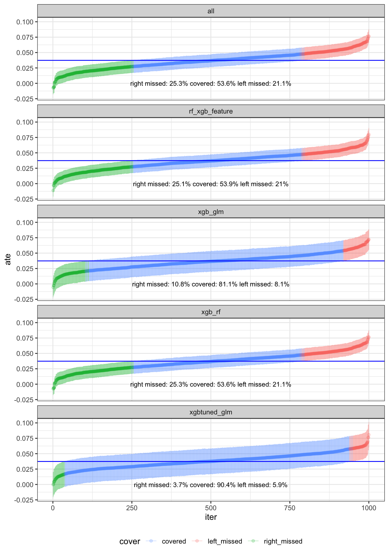
Wow, these are very interesting results! Looking at 1) where we have xgboost, randomforest, glm, and mean, our coverage was pretty horrible at ~50%. For 3) with xgboost and glm, coverage increased to ~80%, very similar to our solo tuned xgboost previously but at least with symmetrical non-coverage, very interesting. But when 2) we combined both xgboost and randomforest, the coverage dropped back to ~50%. Same thing happened when we used feature engineering 4) glmnet prior to xgboost, then couple with xgboost, coverage was only ~50%. But, when we 5) tune xgboost and combine it with glm, coverage increased to ~90%! I was not expecting this result but this is quite amazing! With regards to how long it took for each combination for a quadcore processor with multicore feature:
| method | time_hours |
|---|---|
| SL.xgboost, SL.ranger, SL.glm, SL.mean | 4.02 |
| SL.xgboost, SL.ranger | 4.00 |
| SL.xgboost, SL.glm | 0.47 |
| SL.ranger, SL.xgboost, screen.glmnet | 4.23 |
| tuned SL.xghboost, SL.glm | 3.29 |
Opportunities for improvement
- attempt using optimized hyperparameters for both xgboost and randomforest
- write a function for splitting multicore to several nodes
- try using NNloglik / maximize on auc instead of nnls, would it work better?
- need to test the theory that whether
set.seedworks differently with multicore? Or does future automatically choosesL'Ecuyer-CMRG Algorithm? does our current method ofset.seed(i)of iteration number work ok? - need to try
mcSuperLearner, built-in multicore
Lessons Learnt
- learnt
future_lapply - learnt
multicoreis so much faster!!! Though when wefuture_lapplythe function it appears to have the same time asmultisession - tested
Super Learner, it’s pretty cool! It already has options for parallel computing - found out that mixing flexible model like xgboost (tuned) and logreg regularizes the ensembled model
If you like this article:
- please feel free to send me a comment or visit my other blogs
- please feel free to follow me on BlueSky, twitter, GitHub or Mastodon
- if you would like collaborate please feel free to contact me
- Posted on:
- January 2, 2026
- Length:
- 7 minute read, 1336 words
- Categories:
- r R superlearner xgboost random forest glm nnls tmle
- Tags:
- r R superlearner xgboost random forest glm nnls tmle