My Messy Notes on Building a Super Learner: Peeking Under The Hood of NNLS
By Ken Koon Wong in r R superlearner nnls lawson-hanson
December 21, 2025
📚 Tried building Super Learner from scratch to understand what’s happening under the hood. Walked through the NNLS algorithm step-by-step—turns out ensembling models may beat solo models! Our homegrown version? Surprisingly close to nnls package results ❤️ But, does it really work in real life? 🤷♂️

Motivations
Previously we have learnt the workflow of TMLE and most people would say to use it with Super Learner. But what is Super Learner? The name sounds fancy and cool. Let’s take a look under the hood of how super is this Super Learner. In this blog, we will see what non-negative least square is and what is the algorithm that is behind this method that fuels Super Learner. We’ll take a look at the mathematical procedures and then code from scratch and see if we can reproduce the result. Let’s do this!
Objectives:
- What is Super Learner?
- What is the algorithm behind Super Learner?
- Let’s Put Them All Together
- Opportunities for improvement
- Lessons learnt
What is Super Learner?
Super Learner is an ensemble machine learning algorithm that optimally combines predictions from multiple candidate algorithms to create a single ensembled model. Rather than selecting a single “best” model through traditional model selection methods, Super Learner leverages the strengths of various algorithms by creating a weighted average of their predictions. The fundamental insight is elegant: why choose between a random forest, generalized linear model, or gradient boosting machine when you can let the data determine the optimal combination of all three? This approach was introduced by Mark van der Laan and colleagues and has become particularly popular in causal inference and epidemiology, often paired with Targeted Maximum Likelihood Estimation (TMLE) to obtain robust, efficient estimates of causal effects.
What is the algorithm behind Super Learner?
The beauty of Super Learner lies in its theoretical guarantee: it will perform at least as well as the best single algorithm in your library of candidate learners, and often performs substantially better. This property, known as the oracle inequality, means that Super Learner asymptotically achieves the lowest possible prediction error among the combinations of the candidate algorithms. 🤔 To be transparent, I don’t really understand all these. But, let’s move on. The engine behind this is Non-Negative Least Squares (NNLS), an elegant constrained optimization method that finds the optimal weights for combining your candidate algorithms.
Note: The Super Learner theory does not require NNLS, but works well in practice and is often much faster than true convex combination optimization, and can be seen in the early work on Stacked Regression by Leo Breiman.
NNLS
At its core, NNLS solves a seemingly simple problem: given a matrix X of predictions from your candidate algorithms and an outcome vector y, find weights β that minimize the squared prediction error ||y - Xβ||² subject to two crucial constraints:
- all weights must be non-negative (β ≥ 0)
the weights must sum to one (ensuring a proper convex combination).
Note: Unlike the theoretical Super Learner which requires weights to sum to one (convex combination), NNLS only enforces non-negativity. This relaxation makes the optimization much faster while performing just as well in practice. Thanks to Eric Polley for correcting and educating me on the above. Much appreciated!
Lawson-Hanson Algorithm
The most commonly used algorithm for solving NNLS is the active set method developed by Lawson and Hanson in 1974. This iterative algorithm is remarkably intuitive: it maintains two sets of variables—an “active set” of variables currently in the model with positive weights, and a “passive set” of variables currently excluded (with zero weights). The algorithm begins with all variables in the passive set, then iteratively identifies which passive variable, if added to the active set, would most improve the fit. Once a variable enters the active set, the algorithm solves an unconstrained least squares problem using only the active variables. If any weights become negative during this step, the algorithm removes the most negative variable from the active set and repeats the process. This addition-and-removal dance continues until no passive variables would improve the fit and all active variables have positive weights—at which point we’ve found our optimal solution.
OK, too many words above. Not a fan. 😵💫 Lots of procedures above, let’s break it down to steps and write a simple example with code to go through the process. Let’s create a simple example.
code
X <- rbind(
  c(1.5,3,4),
  c(0.5,2,3),
  c(4.5,6,6)
)

y <- c(2,1,5)
$$ \begin{gather} \text{X} = \begin{bmatrix} 1.5 & 3 & 4 \\ 0.5 & 2 & 3 \\ 4.5 & 6 & 6 \end{bmatrix} ; \text{y} = \begin{bmatrix} 2 \\ 1 \\ 5 \end{bmatrix} \end{gather} $$
Let’s take a quick look at the matrices above. Just glancing at it you would think the weights for each models (columns) should be within column 1 and column 2. Let’s go through Lawson-hanson algorithm procedure
Step 0: Initialize Your Sets
Start with all variables in the passive set (R) and none in the active set (P). Like so:
$$ \text{P} = \emptyset $$
$$ R = \{1, 2, 3\} $$ $$ \beta = \begin{bmatrix} 0 \\ 0 \\ 0 \end{bmatrix} $$
P: Active Set (Take note, I used P as active, not passive; also these are indexes)R: Passive Set (take note, these are indexes)β: weights
We will go throught the iterative procedure below, move Passive set (R) one by one to Active set (P) until we no longer have any passive sets available.
Step 1 Find Gradient
code
# step 1: find gradient
gradient <- t(X) %*% (y-X %*% beta)
if (sum(gradient<=0)==dim(X)[2]) { stop("all gradients are zero or negative, we have achieved optimality") }
if (length(R)==0) { stop("R is empty")}
$$
\begin{gather}
\text{Gradient} = \text{X}^{\text{T}} \cdot (\text{y} - \text{X}\beta)
\end{gather}
$$
The above is the procedure to find gradient for ||y - Xβ||². Let’s put in the numbers and calculate
$$ \begin{gather} \text{Gradient} = \text{X}^{\text{T}} \cdot (\text{y} - \text{X}\beta) \\ = \begin{bmatrix} 1.5 & 3 & 4 \\ 0.5 & 2 & 3 \\ 4.5 & 6 & 6 \end{bmatrix}^\text{T} \cdot ( \begin{bmatrix} 2 \\ 1 \\ 5 \end{bmatrix} - \begin{bmatrix} 1.5 & 3 & 4 \\ 0.5 & 2 & 3 \\ 4.5 & 6 & 6 \end{bmatrix} \begin{bmatrix} 0 \\ 0 \\ 0 \end{bmatrix} ) \\ = \begin{bmatrix} 1.5 & 0.5 & 4.5 \\ 3 & 2 & 6 \\ 4 & 3 & 6 \end{bmatrix} \cdot ( \begin{bmatrix} 2 \\ 1 \\ 5 \end{bmatrix} - \begin{bmatrix} 1.5 & 3 & 4 \\ 0.5 & 2 & 3 \\ 4.5 & 6 & 6 \end{bmatrix} \begin{bmatrix} 0 \\ 0 \\ 0 \end{bmatrix} ) \\ = \begin{bmatrix} 1.5 & 0.5 & 4.5 \\ 3 & 2 & 6 \\ 4 & 3 & 6 \end{bmatrix} \cdot \begin{bmatrix} 2 \\ 1 \\ 5 \end{bmatrix} \\ = \begin{bmatrix} 26.5 \\ 44 \\ 41 \end{bmatrix} \end{gather} $$
Step 2 Check Optimality & Find Next Variable to Add To P
If all gradients are non-positive, we have achieved optimality. If not, proceed to the next step. Find the index of R of the maximum gradient. In this case, max of 26.5, 44, 41 is 44, which is the second column of X.
$$
\begin{gather}
\text{Next Variable} = \text{argmax}_{j \in R} \text{Gradient}_j \\
= 2
\end{gather}
$$
We then move 2 from R (passive set) to P (active set) like so:
$$ \text{P} = \{2\} $$ $$ R = \{1, 3\} $$
Step 3 Solve the Unconstrained Least Squares Problem for Active Set P.
$$ \begin{gather} \beta_P = (\text{X}_P^{\text{T}} \cdot \text{X}_P)^{-1} \cdot \text{X}_P^{\text{T}} \cdot \text{y} \\ = (\begin{bmatrix} 3 \\ 2 \\ 6 \end{bmatrix}^{\text{T}} \cdot \begin{bmatrix} 3 \\ 2 \\ 6 \end{bmatrix})^{-1} \cdot \begin{bmatrix} 3 \\ 2 \\ 6 \end{bmatrix}^{\text{T}} \cdot \begin{bmatrix} 2 \\ 1 \\ 5 \end{bmatrix} \\ = (9 + 4 + 36)^{-1} \cdot \begin{bmatrix} 3 & 2 & 6 \end{bmatrix} \cdot \begin{bmatrix} 2 \\ 1 \\ 5 \end{bmatrix} \\ = 49^{-1} \cdot \begin{bmatrix} 3 \cdot 2 + 2 \cdot 1 + 6 \cdot 5 \end{bmatrix} \\ = 49^{-1} \cdot \begin{bmatrix} 44 \end{bmatrix} \\ = \begin{bmatrix} 0.8979592 \end{bmatrix} \end{gather} $$
Where X_P is the sub-matrix of X containing only the columns in the active set P. In our case, P = {2}, so β is:
$$
\begin{gather}
\beta =
\begin{bmatrix}
0 \\ 0.8979592 \\ 0
\end{bmatrix}
\end{gather}
$$
Still with me? We went from initializing zero weights (beta) for all 3 to now with the second model having weight of 0.89796
Step 4 Check For Negative Weights
$$
\begin{gather}
\text{If any } \beta_P \leq 0, \text{ calculate } \alpha \text{ else go back to step 1}\\
\alpha = \min_{\beta_P \leq 0} \frac{\beta_{old}}{\beta_{old} - \beta_P} \\
\text{If } \alpha < 1, \text{ update } \beta = \beta_{old} + \alpha (\beta_P - \beta_{old}) \\
\text{Remove any variables from P where } \beta \leq 0 \text{ and return them to R}
\end{gather}
$$
Since our weights $\beta$ cannot be negative, and if we hit a negative value, we want to shift all \(\beta\) by \(\alpha\) proportion of the difference and make the calculated negative weight 0 and adjust the other weights equally.
After the above, we go iterate until R set is empty. You get the point, instead of latex the entire calculation, let’s use code to get to our answers.
P <- c()
R <- c(1:dim(X)[2])
beta <- rep(0, dim(X)[2])

while (T) {
# step 1: find gradient
gradient <- t(X) %*% (y-X %*% beta)
if (sum(gradient<=0)==dim(X)[2]) { print("all gradients are zero or negative, we have achieved optimality") ; break }
if (length(R)==0) { print("R is empty") ; break }

# step 2: check optimality
gradient_not_active <- gradient
gradient_not_active[P] <- -Inf
P_x <- which(gradient_not_active==max(gradient_not_active))
P <- c(P,P_x) |> unique() |> sort()
R <- setdiff(R, P_x)

# solve P
beta_i <- beta
beta_i[P] <- solve(t(X[,P]) %*% X[,P]) %*% t(X[,P])%*%y
if (any(beta_i<0)) {
  print(paste0("negative weights: ",paste(beta_i, collapse = " ")))
  idx <- which(beta_i<0)
  beta_old <- beta[idx]
  beta_new <- beta_i[idx]
  alpha <- beta_old/-(beta_new-beta_old)
  beta_i_new <- beta - alpha*(beta-beta_i)
  beta <- beta_i_new |> round(digits = 4)
  print(paste0("new weights after setting negative weight as zero: ", paste(beta,collapse = " ")))
  } else {  beta <- beta_i ; print(beta) }
}
## [1] 0.0000000 0.0000000 0.6721311
## [1] 0.8683544 0.0000000 0.1810127
## [1] "negative weights: 0.666666666666675 0.333333333333364 -7.105427357601e-15"
## [1] "new weights after setting negative weight as zero: 0.6667 0.3333 0"
## [1] "R is empty"
beta
## [1] 0.6667 0.3333 0.0000
X %*% beta
##         [,1]
## [1,] 1.99995
## [2,] 0.99995
## [3,] 4.99995
Wow, it worked! Look at our weights (beta) and our final results! As suspected, column 1 and 2 will have the weights (more on column 1) and when combined our final numbers are quite close to our y, which is 2, 1, 5 . Awesome! Now, let’s simulate more data and see if our code works and compare it with nnls package!
Let’s Put Them All Together
Simulate Data
# labels/outcome/y
num_labels <- 1000
label_range <- 1:5
y <- sample(label_range, num_labels, replace=T)

# X matrix
num_models <- 5
X <- matrix(nrow = num_labels, ncol = num_models)
for (i in 1:num_models) {
  sd <- sample(c(0.01,1,10))
  for (j in 1:num_labels) {
  X[j, i] <- rnorm(1, mean = y[j], sd = sd)
}
}
Alright, what we did above is basically simulated y and X
P <- c()
R <- c(1:dim(X)[2])
beta <- rep(0, dim(X)[2])

while (T) {
# step 1: find gradient
gradient <- t(X) %*% (y-X %*% beta)
if (sum(gradient<=0)==dim(X)[2]) { print("all gradients are zero or negative, we have achieved optimality") ; break }
if (length(R)==0) { print("R is empty") ; break }

# step 2: check optimality
gradient_not_active <- gradient
gradient_not_active[P] <- -Inf
P_x <- which(gradient_not_active==max(gradient_not_active))
P <- c(P,P_x) |> unique() |> sort()
R <- setdiff(R, P_x)

# solve P
beta_i <- beta
beta_i[P] <- solve(t(X[,P]) %*% X[,P]) %*% t(X[,P])%*%y
if (any(beta_i<0)) {
  print(paste0("negative weights: ",paste(beta_i, collapse = " ")))
  idx <- which(beta_i<0)
  beta_old <- beta[idx]
  beta_new <- beta_i[idx]
  alpha <- beta_old/-(beta_new-beta_old)
  beta_i_new <- beta - alpha*(beta-beta_i)
  beta <- beta_i_new |> round(digits = 4)
  print(paste0("new weights after setting negative weight as zero: ", paste(beta,collapse = " ")))
  } else {  beta <- beta_i ; print(beta) }
}
## [1] 0.000000 0.000000 1.000061 0.000000 0.000000
## [1] 1.289716e-05 0.000000e+00 1.000049e+00 0.000000e+00 0.000000e+00
## [1] "negative weights: -4.80441441441621e-06 0 0.530291436850037 0 0.469820844889452"
## [1] "new weights after setting negative weight as zero: 0 0 0.6578 0 0.3423"
## [1] "negative weights: -4.57899476983191e-06 6.81265663325082e-05 0.530205009482599 0 0.469839806590533"
## [1] "new weights after setting negative weight as zero: 0 0 0.6578 0 0.3423"
## [1] "negative weights: -4.73337830228063e-06 6.51033708645959e-05 0.530467184328906 -5.88823524796493e-06 0.469586269810267"
## Warning in alpha * (beta - beta_i): longer object length is not a multiple of
## shorter object length
## [1] "new weights after setting negative weight as zero: 0 0 0.6578 0 0.3423"
## [1] "R is empty"
Let’s look at our weights and RMSE
beta
## [1] 0.0000 0.0000 0.6578 0.0000 0.3423
sqrt(mean((y - X %*% beta)^2))
## [1] 0.007206879
Let’s look at nnls package and see if we can the same result
model <- nnls::nnls(A=X,b=y)
model
## Nonnegative least squares model
## x estimates: 0 6.970084e-05 0.53029 0 0.4697488
## residual sum-of-squares: 0.04886
## reason terminated: The solution has been computed sucessfully.
sqrt(mean((y - X %*% model$x)^2))
## [1] 0.006989728
wow! Awesome!!! Looks the same or at least very similar. Alright, now we’re at least able to reproduce the nnls portion from scratch. Let’s see if we can simulate a non-linear data and train with different models and see how our end result is!
Let’s Super Learn this thing
Click below at code to expand for the entire procedures. We basically ran 3 different models in tidymodels, linear regression, xgboost, and random forest with recipe (y ~ .), not specifying any interaction/polynomial relationships for a simulated data below.
n <- 1000
x <- rnorm(n)
w <- rnorm(n, 0.5*x)
y <- 0.2*x + 0.5*w + 0.2*x*w + 0.05*x^2
Made sure to set seed for reproducibility, create 5 fold for cross validation. Then extract all the prediction for validation sets from each models and stack them into X matrix. Then extract the RMSE from each models and stack them into metrics matrix. Finally, we run our nnls code above to get the weights and RMSE for super learner. We repeat this for 1000 iterations and log the results.
This cross-validation step is the defining feature of the Super Learner. By fitting each base learner on training folds and generating out-of-fold predictions, we obtain an unbiased prediction matrix that is then used to estimate optimal ensemble weights via NNLS.
code
library(tidymodels)
library(future)
library(furrr)

# Set up parallel processing
plan(multisession, workers = availableCores() - 2)

# Define the function to run for each iteration
run_iteration <- function(i) {
  set.seed(i)
  n <- 1000
  x <- rnorm(n)
  w <- rnorm(n, 0.5*x)
  y <- 0.2*x + 0.5*w + 0.2*x*w + 0.05*x^2

  df <- tibble(x,w,y)
  split <- initial_split(df)
  train <- training(split)
  test <- testing(split)
  # preprocess
  rec <- recipe(y ~ ., data=train)

  # linear regression
  lr_spec <- linear_reg()
  wf <- workflow() |>
    add_recipe(rec) |>
    add_model(lr_spec)
  folds <- vfold_cv(train, 5)
  cv_results <- wf |>
    fit_resamples(folds, control = control_resamples(save_pred = TRUE))
  cv_metrics <- collect_metrics(cv_results) |> filter(.metric == "rmse") |> pull(mean)
  cv_preds <- collect_predictions(cv_results)

  #xgboost
  xgb_spec <- boost_tree(engine = "xgboost", mode = "regression")
  wf <- workflow() |>
    add_recipe(rec) |>
    add_model(xgb_spec)
  cv_results <- wf |>
    fit_resamples(folds, control = control_resamples(save_pred = T))
  cv_metrics2 <- collect_metrics(cv_results) |> filter(.metric == "rmse") |> pull(mean)
  cv_preds2 <- collect_predictions(cv_results)

  # random forest
  rf_spec <- rand_forest(mode = "regression")
  wf <- workflow() |>
    add_recipe(rec) |>
    add_model(rf_spec)
  cv_results <- wf |>
    fit_resamples(folds, control = control_resamples(save_pred = T))
  cv_metrics3 <- collect_metrics(cv_results) |> filter(.metric == "rmse") |> pull(mean)
  cv_preds3 <- collect_predictions(cv_results) |>
    mutate(model = "rf")
  X <- cbind(cv_preds |> select(X1=.pred),cv_preds2 |> select(X2=.pred), cv_preds3 |> select(X3=.pred)) |> as.matrix()
  y <- cv_preds |> select(y) |> as.matrix()
  metrics <- cbind(cv_metrics,cv_metrics2,cv_metrics3)

  # nnls
  P <- c()
  R <- c(1:dim(X)[2])
  beta <- rep(0, dim(X)[2])

  while (T) {
    # step 1: find gradient
    gradient <- t(X) %*% (y-X %*% beta)
    if (sum(gradient<=0)==dim(X)[2]) { print("all gradients are zero or negative, we have achieved optimality") ; break }
    if (length(R)==0) { print("R is empty") ; break }
    # step 2: check optimality
    gradient_not_active <- gradient
    gradient_not_active[P] <- -Inf
    P_x <- which(gradient_not_active==max(gradient_not_active))
    P <- c(P,P_x) |> unique() |> sort()
    R <- setdiff(R, P_x)
    # solve P
    beta_i <- beta
    beta_i[P] <- solve(t(X[,P]) %*% X[,P]) %*% t(X[,P])%*%y
    if (any(beta_i<0)) {
      print(paste0("negative weights: ",paste(beta_i, collapse = " ")))
      idx <- which(beta_i<0)
      beta_old <- beta[idx]
      beta_new <- beta_i[idx]
      alpha <- beta_old/-(beta_new-beta_old)
      beta_i_new <- beta - alpha*(beta-beta_i)
      beta <- beta_i_new |> round(digits = 4)
      print(paste0("new weights after setting negative weight as zero: ", paste(beta,collapse = " ")))
    } else {  beta <- beta_i ; print(beta) }
  }

  rmse_superlearner <- sqrt(mean((y - X %*% beta)^2))
  rmse_result <- if (sum(metrics < rmse_superlearner) >= 1) { "solo_better" } else { "superlearner_better" }

  model <- nnls::nnls(A=X,b=y)
  rmse_ours_nnls <- c(rmse_superlearner, sqrt(mean((y - X %*% model$x)^2)))
  same_weights_result <- if (sum(round(beta, 4) == round(model$x, 4)) == 3) { "same" } else { "not_same" }
  weights_log <- c(model$x, beta)

  return(list(rmse_log = rmse_result, same_weights_log = same_weights_result, weights_log=weights_log))
}

# Run with future_map
results <- future_map(1:1000, run_iteration, .options = furrr_options(seed = TRUE), .progress = TRUE)
Let’s Compare RMSE of Solo models vs Super Learner models
code
library(tidyverse)

# Extract results
rmse_log <- map_chr(results, "rmse_log")
same_weights_log <- map_chr(results, "same_weights_log")
weight_logs <- matrix(NA, ncol = 6, nrow = 1000)
for (i in 1:1000) {
  weight_logs[i, 1:6] <- results[[i]]$weights_log
}

plotrmse_log <- tibble(rmse=rmse_log) |>
  ggplot(aes(x=rmse)) +
  geom_bar() +
  theme_bw()
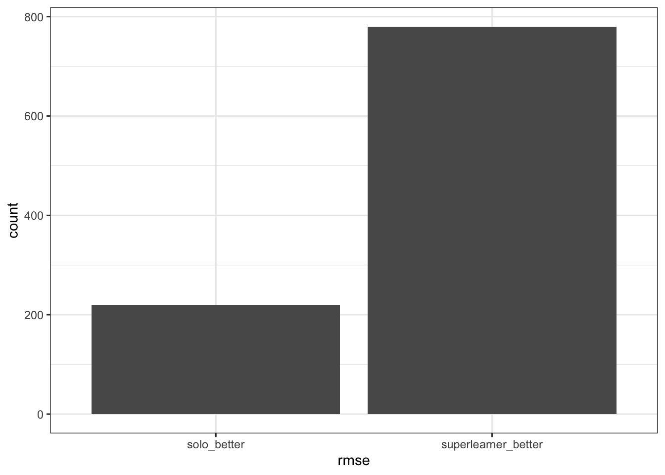
Wow, look at that! superlearner/ensembled model does appear to have better RMSE compared to solo models! Let’s take a look and see if our noob nnls from scratch is comparable with nnls package.
Comparing Our NNLS to nnls package
code
plotsameweights <- tibble(same_weights=same_weights_log) |>
  ggplot(aes(x=same_weights)) +
  geom_bar() +
  theme_bw()
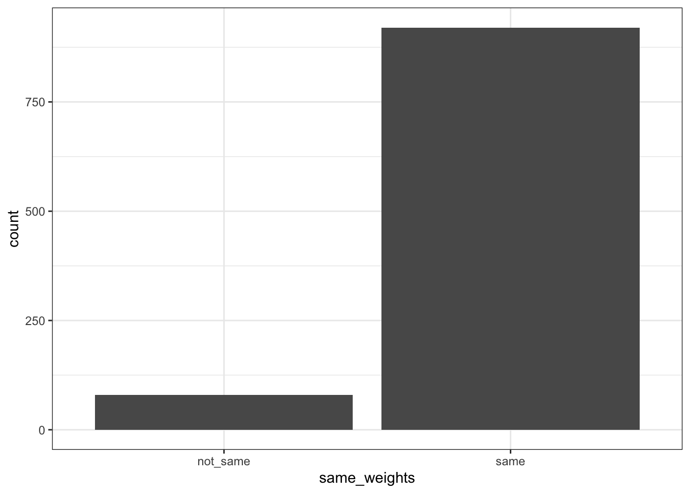
Wow, most of the weights are the same if we round up to 4 digits! Let’s check on the ones with difference, is it REALLY that different?
code
plotdiff123 <- weight_logs |>
  as_tibble() |>
  mutate(diff1 = round(V4-V1, 4),
         diff2 = round(V5-V2, 4),
         diff3 = round(V6-V3, 4),
         sum_diff = diff1+diff2+diff3) |>
  filter(sum_diff != 0) |>
  pivot_longer(cols = c(diff1,diff2,diff3), names_to = "diff", values_to = "values") |>
  ggplot(aes(x=values,fill=diff)) +
  geom_histogram(position = "dodge2") +
  theme_bw()
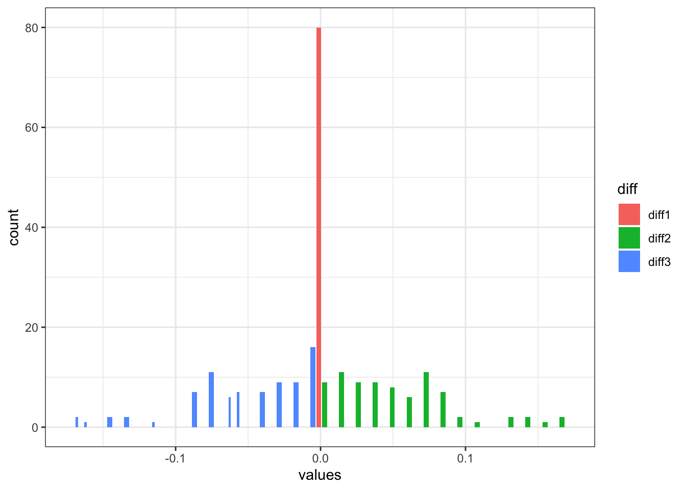
This makes sense, most of the differences are between xgboost (diff2) and random forest (diff3), as our linear regression (diff1) model without correct specification probably won’t have a whole of contributions, hence if there is a difference between our algorithm and nnls, it would be minimal (center in red). It also make sense that if there is a difference in xgboost or random forest model, we would see different weight on the other model contribution. Now the question is, with these weight differences, does it make a huge difference in RMSE? I suspect not so much.
code
rmse_compare <- matrix(NA, ncol = 2, nrow = 1000)
for (i in 1:1000) {
  rmse_compare[i,1:2] <- results[[i]]$rmse_ours_nnls
}

plotcompare <- weight_logs |>
  as_tibble() |>
  mutate(row = row_number()) |>
  mutate(diff1 = round(V4-V1, 4),
         diff2 = round(V5-V2, 4),
         diff3 = round(V6-V3, 4),
         sum_diff = diff1+diff2+diff3) |>
  filter(sum_diff != 0) |>
  left_join(as_tibble(rmse_compare) |>
              mutate(row = row_number()), by = "row") |>
  mutate(V1.y = round(V1.y, 4),
         V2.y = round(V2.y, 4)) |>
  mutate(check = case_when(
    V1.y == V2.y ~ "same",
    V1.y < V2.y ~ "our_nnls_better",
    V1.y > V2.y ~ "nnls_package_better",
    TRUE ~ NA_character_
  )) |>
  ggplot(aes(x=check)) +
  geom_bar() +
  theme_bw()
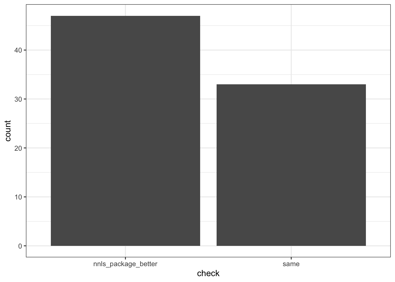
lol, nnls package clearly is better than our home-grown algorithm! But by how much?
code
plotdiffrmse <- weight_logs |>
  as_tibble() |>
  mutate(row = row_number()) |>
  mutate(diff1 = round(V4-V1, 4),
         diff2 = round(V5-V2, 4),
         diff3 = round(V6-V3, 4),
         sum_diff = diff1+diff2+diff3) |>
  filter(sum_diff != 0) |>
  left_join(as_tibble(rmse_compare) |>
              mutate(row = row_number()), by = "row") |>
  mutate(V1.y = round(V1.y, 4),
         V2.y = round(V2.y, 4)) |>
  mutate(diff_rmse = V1.y - V2.y) |>
  ggplot(aes(diff_rmse)) +
  geom_histogram() +
  theme_bw()
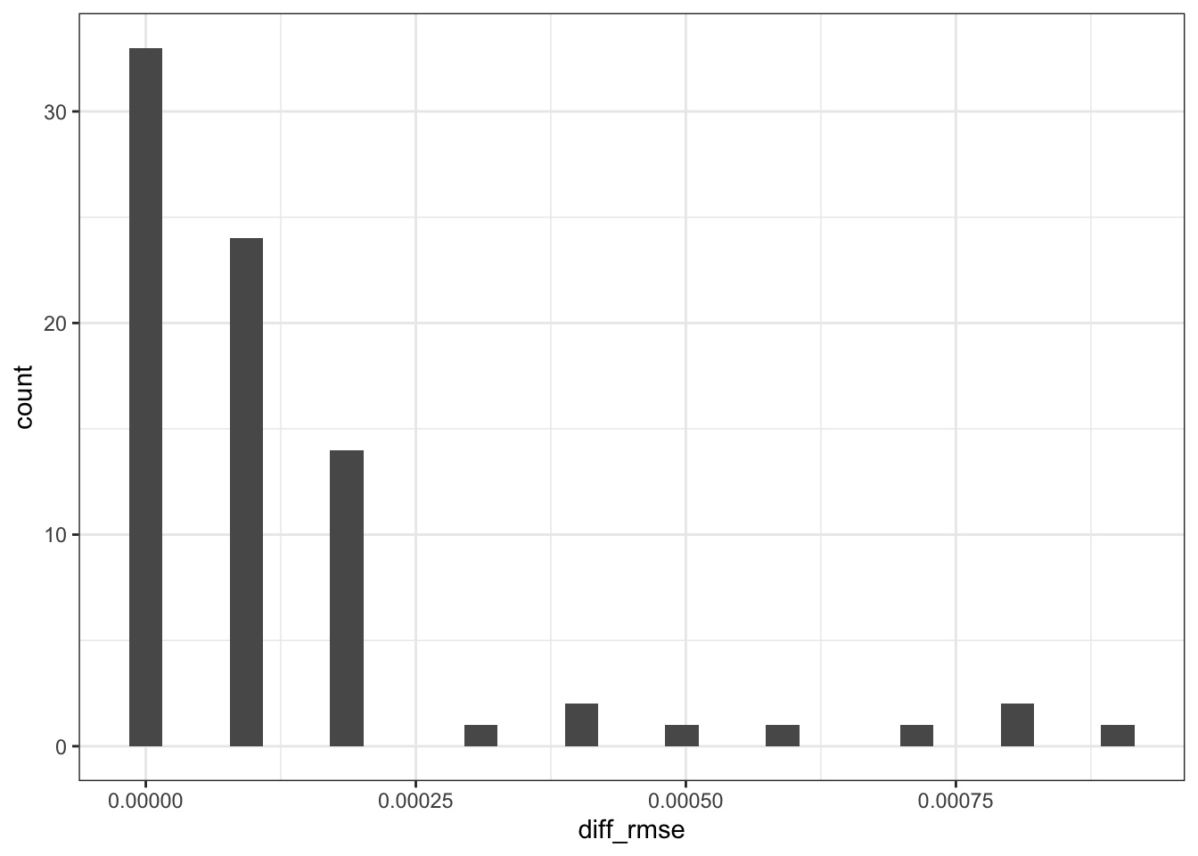
😵💫 It’s really not that much different! Let’s find the max.
code
weight_logs |>
  as_tibble() |>
  mutate(row = row_number()) |>
  mutate(diff1 = round(V4-V1, 4),
         diff2 = round(V5-V2, 4),
         diff3 = round(V6-V3, 4),
         sum_diff = diff1+diff2+diff3) |>
  filter(sum_diff != 0) |>
  left_join(as_tibble(rmse_compare) |>
              mutate(row = row_number()), by = "row") |>
  mutate(V1.y = round(V1.y, 4),
         V2.y = round(V2.y, 4)) |>
  mutate(diff_rmse = V1.y - V2.y) |>
  pull(diff_rmse) |> max()
## [1] 9e-04
## [1] 9e-04
🥹 Does that mean our home-grown algorithm works just as well? You be the judge. Let me know if this is due to pure luck!
Acknowledgement:
Thanks Eric Polley for correcting and educating me on that NNLS does not require the beta coefficients sum up to 1 (only non-negative). Also The Super Learner theory does not require NNLS, but works well in practice and is often much faster than true convex combination optimization, and can be seen in the early work on Stacked Regression by Leo Breiman. Much appreciated!
Opportunities for improvement
- will try multicore sometime in the future, is it really faster than multisession?
- need to learn/figure out FAST nnls algorithm which I believe
nnlspackage uses - need to venture more in parallel computing
- compare with the actual
SuperLearnerpackage
Lessons learnt
- learnt to build Super Learner using non-negative least square model
- learnt Lawson-Hanson algorithm and how it’s implemented, compared with
nnlsand results not too shabby! - learnt some basics of parallel computing
If you like this article:
- please feel free to send me a comment or visit my other blogs
- please feel free to follow me on BlueSky, twitter, GitHub or Mastodon
- if you would like collaborate please feel free to contact me
- Posted on:
- December 21, 2025
- Length:
- 17 minute read, 3574 words
- Categories:
- r R superlearner nnls lawson-hanson
- Tags:
- r R superlearner nnls lawson-hanson