From Complete Separation To Maximum Likelihood Estimation in Logistic Regresion: A Note To Myself
By Ken Koon Wong in r R hessian maximum likelihood estimation derivative chain rule quotient rule optim mle complete separation
May 17, 2025
Refreshed my rusty calculus skills lately! 🤓 Finally understand what happens during complete separation and why those coefficient SE get so extreme. The math behind maximum likelihood estimation makes more sense now! Chain rule, quotient rule, matrix inversion are crucial!

Objectives:
- A Complete Separation
- Wait, How Do We Even Estimate The Coefficient?
- Let’s Inspect Complete Separation with Optim
- Final Thoughts
- Lessons Learnt
A Complete Separation
I know this is a rather basic concept, but I just recently came across this interesting problem. Complete separation in logistic regression occurs when a predictor perfectly divides your outcomes into groups - like if all patients over 50 developed a condition and none under 50 did. This creates a problem because the model tries to draw an impossibly steep line at that boundary, causing coefficient estimates to become unreliable and extremely large. It’s a case where perfect prediction paradoxically breaks the statistical machinery, making the model unable to properly quantify uncertainty or provide stable estimates.
Let’s Code
y <- c(rep(1,50),rep(0,50))
x <- c(rep(0,50),rep(1,50))

model <- glm(y~x, family="binomial")
summary(model)
##
## Call:
## glm(formula = y ~ x, family = "binomial")
##
## Coefficients:
##             Estimate Std. Error z value Pr(>|z|)
## (Intercept)    26.57   50363.44   0.001    1.000
## x             -53.13   71224.73  -0.001    0.999
##
## (Dispersion parameter for binomial family taken to be 1)
##
##     Null deviance: 1.3863e+02  on 99  degrees of freedom
## Residual deviance: 5.8016e-10  on 98  degrees of freedom
## AIC: 4
##
## Number of Fisher Scoring iterations: 25
A few reminder for myself, if I see these things on a logistic regression model, think about separation:
Warning: glm.fit: algorithm did not convergeandfitted probabilities numerically 0 or 1 occurred- Extreme value for
estimates. Imagine trying toexpcoefficient of x, odds ratio would 8.4141037\times 10^{-24} which is a very very small. - Enormouse standard errors
- Residual deviance very very small, almost 0. Indicating model fit perfectly
- Number of Fisher Scoring Iteration reaching max iteration, indicating the model is not converging
Let’s take a look for a normal logistic regression model summary look like.
x <- runif(100,0,1)
y <- rbinom(100, 1, plogis(2*x))

model <- glm(y~x, family="binomial")
summary(model)
##
## Call:
## glm(formula = y ~ x, family = "binomial")
##
## Coefficients:
##             Estimate Std. Error z value Pr(>|z|)
## (Intercept)   0.1989     0.4677   0.425   0.6707
## x             1.7392     0.8823   1.971   0.0487 *
## ---
## Signif. codes:  0 '***' 0.001 '**' 0.01 '*' 0.05 '.' 0.1 ' ' 1
##
## (Dispersion parameter for binomial family taken to be 1)
##
##     Null deviance: 114.61  on 99  degrees of freedom
## Residual deviance: 110.59  on 98  degrees of freedom
## AIC: 114.59
##
## Number of Fisher Scoring iterations: 4
Look at the difference in the summary output. The estimates are much smaller, and the standard errors are reasonable. The residual deviance is also much larger, indicating that the model is not perfectly fitting the data. Also with lower iterations.
This made me really curious how does glm find these coefficients to begin with? Yes, I’ve heard of maximum likelihood estimation and I know that it uses that to find the estimate and standard error, but… how does it actually do that? 🤔
Also, if we have a perfect prediction, shouldn’t our standard error be very very small instead of very very big !?! Maybe the answer lies in how these coefficients are estimated!
Wait, How Do We Even Estimate The Coefficient?
- Choose a distribution from the exponential family (binomial for logistic regression, Poisson for count data, etc.)
- Specify a link function that connects the linear predictor to the response variable (logit link for logistic regression)
- Construct the likelihood function based on the chosen distribution - this represents the probability of observing your data given the parameters
- Find the maximum likelihood estimates (MLEs) by:
- Taking the log of the likelihood function (for mathematical convenience)
- Finding the derivatives with respect to each coefficient
- Setting these derivatives equal to zero
- Solving for the coefficients that maximize the likelihood
- Since most GLMs don’t have closed-form solutions, the model uses iterative numerical methods (like Fisher Scoring or Newton-Raphson) to converge to the maximum likelihood estimates
Alright, let’s go through step by step. As for the first step, we’re going to choose a binomial distribution. For simplicity, our model only has intercept and one predictor.
Link function
\begin{gather} \text{logit}(p_i) = \log\left(\frac{p_i}{1-p_i}\right) = \beta_0 + \beta_1 x_{1i} = \text{z} \end{gather}
this is basically the equation for log odds, and we will use z
Probability function
\begin{gather} p_i = \frac{1}{1 + e^{-z}} \ = \frac{1}{1 + e^{-(\beta_0 + \beta_1 x_{1i})}} \end{gather}
Construct the likelihood function
\begin{gather} L(\boldsymbol{\beta_0, \beta_1}) = \prod_{i=1}^{n} p_i^{y_i} (1-p_i)^{1-y_i} \ \end{gather}
Notice that if y_i is 1, the first term will be 1 and the second term will be 0. If y_i is 0, the first term will be 0 and the second term will be 1. This is very convenient! And the likelihood function is a product of the probabilities of each observation. We essentially want to maximize this likelihood function. We want to find the coefficients that make the observed data most probable.
Log-likelihood function
$$ \begin{gather} \ln L(\boldsymbol{\beta_0, \beta_1}) \ = \sum_{i=1}^{n} \left[ y_i \ln(p_i) + (1-y_i) \ln(1-p_i) \right] \end{gather} $$
The reason for taking the log is that it turns products into sums, which are easier to work with mathematically. Also notice that we use natural log here.
Derivative With Respect To Coefficient
Let’s look at b0 the intercept first. The final answer should be:
$$
\begin{gather}
\frac{\partial \ln L(\boldsymbol{\beta_0, \beta_1})}{\partial \beta_0} = \sum_{i=1}^{n} \left( y_i - p_i \right)
\end{gather}
$$
As for b1 the coefficient of the predictor, the final answer should be:
$$
\begin{gather}
\frac{\partial \ln L(\boldsymbol{\beta_0, \beta_1})}{\partial \beta_1} = \sum_{i=1}^{n} \left( y_i - p_i \right) x_{1i}
\end{gather}
$$
Let’s try to practice our mathematical muscles and try to proof both of these equations.
Intercept
$$ \begin{gather} \frac{\partial \ln L(\boldsymbol{\beta_0, \beta_1})}{\partial \beta_0} = \frac{\partial}{\partial \beta_0} \sum_{i=1}^{n} \left[ y_i \ln(p_i) + (1-y_i) \ln(1-p_i) \right] \newline = \sum_{i=1}^{n} \frac{\partial}{\partial \beta_0} \left[ y_i \ln(p_i) + (1-y_i) \ln(1-p_i) \right] \newline = \sum_{i=1}^{n} \left[ y_i \frac{1}{p_i} \frac{\partial p_i}{\partial \beta_0} + (1-y_i) \frac{1}{1-p_i} \frac{\partial (1-p_i)}{\partial \beta_0} \right] \end{gather} $$
Since there are 2 parts, let’s work on the left part first. $$ \begin{gather} y_i \frac{\partial}{\partial \beta_0} \ln(p_i) \newline = y_i \frac{1}{p_i} \frac{\partial p_i}{\partial \beta_0} \newline = y_i \frac{1}{p_i} \frac{\partial}{\partial \beta_0} \left( \frac{1}{1 + e^{-z}} \right) \newline = y_i \frac{1}{p_i} \frac{\partial}{\partial \beta_0} \left( \frac{1}{1 + e^{-(\beta_0 + \beta_1 x_{1i})}} \right) \end{gather} $$
Alright, let’s focus on the derivative of the probability function. We can use the quotient rule here. $$ \begin{gather} \frac{\partial}{\partial \beta_0} \left( \frac{1}{1 + e^{-(\beta_0 + \beta_1 x_{1i})}} \right) \newline = -\frac{(1 + e^{-(\beta_0 + \beta_1 x_{1i})}) \cdot \frac{\partial}{\partial \beta_0} 1 - 1 \cdot \frac{\partial}{\partial \beta_0} (1 + e^{-(\beta_0 + \beta_1 x_{1i})})} {(1 + e^{-(\beta_0 + \beta_1 x_{1i})})^2} \newline = -\frac{(1 + e^{-(\beta_0 + \beta_1 x_{1i})}) \cdot 0 - 1 \cdot (0 + e^{-(\beta_0 + \beta_1 x_{1i})} \cdot -1)} {(1 + e^{-(\beta_0 + \beta_1 x_{1i})})^2} \newline = \frac{e^{-(\beta_0 + \beta_1 x_{1i})}} {(1 + e^{-(\beta_0 + \beta_1 x_{1i})})^2} \end{gather} $$
Let’s put all the left part together.
$$ \begin{gather} y_i \frac{1}{p_i} \left( \frac{e^{-(\beta_0 + \beta_1 x_{1i})}} {(1 + e^{-(\beta_0 + \beta_1 x_{1i})})^2} \right) \newline = y_i (1 + e^{-(\beta_0 + \beta_1 x_{1i})}) \left( \frac{e^{-(\beta_0 + \beta_1 x_{1i})}} {(1 + e^{-(\beta_0 + \beta_1 x_{1i})})^2} \right) \newline = y_i \left( \frac{e^{-(\beta_0 + \beta_1 x_{1i})}} {1 + e^{-(\beta_0 + \beta_1 x_{1i})}} \right) \end{gather} $$
Alright, now let’s work on the right part. $$ \begin{gather} (1-y_i) \frac{\partial}{\partial \beta_0} \ln(1-p_i) \newline = (1-y_i) \frac{1}{1-p_i} \frac{\partial (1-p_i)}{\partial \beta_0} \newline = (1-y_i) \frac{1}{1-p_i} \frac{\partial}{\partial \beta_0} \left( 1 - \frac{1}{1 + e^{-(\beta_0 + \beta_1 x_{1i})}} \right) \newline = (1-y_i) \frac{1}{1-p_i} \left( 0 - \frac{e^{-(\beta_0 + \beta_1 x_{1i})}} {(1 + e^{-(\beta_0 + \beta_1 x_{1i})})^2} \right) \newline = (1-y_i) \frac{1 + e^{-(\beta_0 + \beta_1 x_{1i})}}{e^{-(\beta_0 + \beta_1 x_{1i})}} \left( -\frac{e^{-(\beta_0 + \beta_1 x_{1i})}} {(1 + e^{-(\beta_0 + \beta_1 x_{1i})})^2} \right) \newline = -\frac{1-y_i}{1 + e^{-(\beta_0 + \beta_1 x_{1i})}} \end{gather} $$
A note to myself, for line 26, we used the answer on line 22 to replace the derivative.
Okay, still with me? Let’s put them all together! $$ \begin{gather} \sum_{i=1}^{n} \left[ y_i \frac{1}{p_i} \frac{\partial p_i}{\partial \beta_0} + (1-y_i) \frac{1}{1-p_i} \frac{\partial (1-p_i)}{\partial \beta_0} \right] \newline = \sum_{i=1}^{n} \left[ y_i \left( \frac{e^{-(\beta_0 + \beta_1 x_{1i})}} {1 + e^{-(\beta_0 + \beta_1 x_{1i})}} \right) + \frac{-(1-y_i)}{1 + e^{-(\beta_0 + \beta_1 x_{1i})}}\right] \newline = \sum_{i=1}^{n} \left[ \frac{e^{-(\beta_0 + \beta_1 x_{1i})} y_i - 1 + y_i }{1+e^{-(\beta_0 + \beta_1 x_{1i})}}\right] \newline = \sum_{i=1}^{n} \left[ \frac{y_i (1 + e^{-(\beta_0 + \beta_1 x_{1i})}) - 1}{1 + e^{-(\beta_0 + \beta_1 x_{1i})}}\right] \newline = \sum_{i=1}^{n} \left[ \frac{y_i (1 + e^{-(\beta_0 + \beta_1 x_{1i})}) }{1 + e^{-(\beta_0 + \beta_1 x_{1i})}} - \frac{1}{1 + e^{-(\beta_0 + \beta_1 x_{1i})}}\right] \newline = \sum_{i=1}^{n} \left[ y_i - p_i\right] \end{gather} $$
YES !!! WE DID IT !!! It was a really good time to refresh on my calculus. Especially on
chain rule, quotient rule. As for the coefficient of x1 it’s essentially the same process as above, and we will get to the derivative mentioned earlier if we work it out. We will spare that process on this blog.
Since we know the derivative of the log-likelihood function, let’s create a gradient descent function to find the coefficients. Let’s code it!
Code
# Custom gradient descent function for logistic regression
grad_beta0_vec <- grad_beta1_vec <- c()

logistic_gradient_descent <- function(x, y, learning_rate = 0.01, max_iter = 100000, tol = 1e-6) {
  # Initialize parameters
  beta0 <- 0
  beta1 <- 0

  # Store history for tracking convergence
  history <- matrix(0, nrow = max_iter, ncol = 2)

  for (i in 1:max_iter) {
    # Calculate predicted probabilities with current parameters
    linear_pred <- beta0 + beta1 * x
    p <- 1 / (1 + exp(-linear_pred))

    # Calculate gradients (derivatives of log-likelihood)
    grad_beta0 <- sum(y - p)
    grad_beta1 <- sum((y - p) * x)

    # records grad for visualization
    grad_beta0_vec[i] <<- grad_beta0
    grad_beta1_vec[i] <<- grad_beta1

    # Store current parameters
    history[i, ] <- c(beta0, beta1)

    # Update parameters using gradient ascent (since we want to maximize log-likelihood)
    beta0_new <- beta0 + learning_rate * grad_beta0
    beta1_new <- beta1 + learning_rate * grad_beta1

    # Check for convergence
    if (abs(beta0_new - beta0) < tol && abs(beta1_new - beta1) < tol) {
      # Trim history to actual iterations used
      history <- history[1:i, ]
      break
    }

    # Update parameters
    beta0 <- beta0_new
    beta1 <- beta1_new

  }

  # Calculate final log-likelihood
  linear_pred <- beta0 + beta1 * x
  p <- 1 / (1 + exp(-linear_pred))
  log_lik <- sum(y * log(p) + (1 - y) * log(1 - p))

  # Return results
  return(list(
    par = c(beta0, beta1),
    iterations = nrow(history),
    convergence = if(i < max_iter) 0 else 1,
    history = history,
    log_likelihood = log_lik
  ))
}

# Run the custom gradient descent function
n <- 1000
x <- runif(n, 0, 1)
y <- rbinom(n, 1, plogis(0.5 + 2*x))

result_custom <- logistic_gradient_descent(x, y)

# Print results
cat(paste0("Final parameter estimates:\n",
             "Beta0: ", round(result_custom$par[1], 4), " (True: 0.5)\n",
             "Beta1: ", round(result_custom$par[2], 4), " (True: 2)\n",
             "Converged in ", result_custom$iterations, " iterations\n",
             "Final log-likelihood: ", round(result_custom$log_likelihood, 4)))
## Final parameter estimates:
## Beta0: 0.4365 (True: 0.5)
## Beta1: 1.9399 (True: 2)
## Converged in 115 iterations
## Final log-likelihood: -485.1456
Not too shabby! Let’s visualize our coefficients
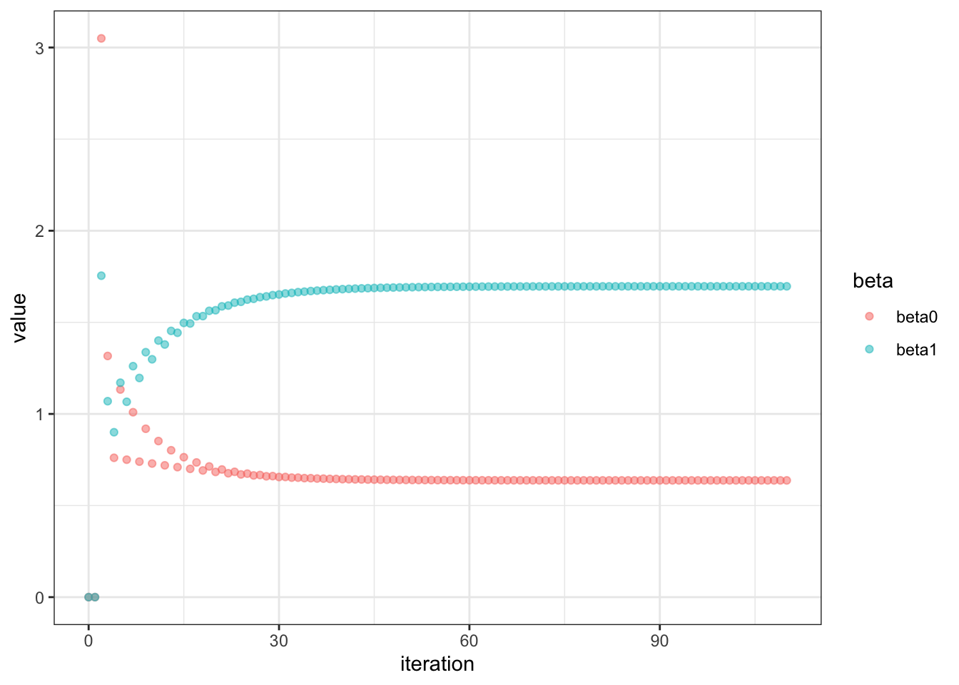
Let’s visualize our gradients, our derivatives with respect to beta0 and beta1
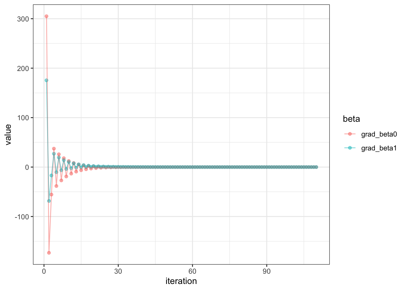
This is great, you can see that the first few iterations, there were wide gradients, but then it quickly converges to a small gradient.
Alternatively you can just use likelihood function and optim to find the coefficients like so.
n <- 1000
x <- runif(n,0,1)
y <- rbinom(n, 1, plogis(0.5 + 2*x))

log_likelihood <- function(param, x, y) {
  beta0 <- param[1]
  beta1 <- param[2]
  p <- 1 / (1 + exp(-(beta0 + beta1 * x)))
  return(-sum(y * log(p) + (1 - y) * log(1 - p)))
}

gradient <- function(param, x, y) {
  beta0 <- param[1]
  beta1 <- param[2]
  p <- 1 / (1 + exp(-(beta0 + beta1 * x)))

  # Negated derivatives (since we're minimizing)
  d_beta0 <- -sum(y - p)
  d_beta1 <- -sum((y - p) * x)

  return(c(d_beta0, d_beta1))
}

(result <- optim(
  par = c(0, 0),
  fn = log_likelihood,
  gr = gradient,
  x = x,
  y = y,
  method = "BFGS",
  hessian = TRUE
))
## $par
## [1] 0.3549094 2.3746947
##
## $value
## [1] 458.7256
##
## $counts
## function gradient
##       24       11
##
## $convergence
## [1] 0
##
## $message
## NULL
##
## $hessian
##           [,1]     [,2]
## [1,] 145.81103 58.28458
## [2,]  58.28458 33.50235
OK, something we need to note here is that the optim function minimizes the function, while we want to maximize the log-likelihood function. So we need to negate the log-likelihood function and the gradient, hence you see the return of - in both the logistic regression function and gradient. This means that the original Hessian matrix should be multiplied by -.
(hessian_matrix <- -result$hessian)
##            [,1]      [,2]
## [1,] -145.81103 -58.28458
## [2,]  -58.28458 -33.50235
Now, because according to Fisher Information:
$$
\begin{gather}
I(\theta) = -E\left[\frac{\partial^2 \ln L(\theta)}{\partial \theta^2}\right]
\end{gather}
$$
The \(I(\theta)\) here represents Fisher Information, not identity matrix. We see that there is a - in front of the equation, hence the ultimate Hessian matrix calculated by optim is actually the Fisher Information.
The interesting thing too is this works without actually specifying the gradient. OK, now we’ve estimated the coefficients, what about the standard error? And also what’s Hessian matrix you say? Let’s take a look!
Hessian Matrix
A Hessian matrix is a square matrix of second-order partial derivatives of a scalar-valued function. For a function f(x₁, x₂, …, xₙ) with n variables, the Hessian is an n×n matrix where each element Hij is the second partial derivative of f with respect to xi and xj.
For simplicity, we will use the log likelihood function \(\ln L(\beta_0,\beta_1)\) , and it would be second derivative of the log-likelihood function with respect to the coefficients \(\beta_0 , \beta_1\).
$$ \begin{bmatrix} \frac{\partial^2 \ln L}{\partial \beta_0^2} & \frac{\partial^2 \ln L}{\partial \beta_0 \partial \beta_1} \newline \frac{\partial^2 \ln L}{\partial \beta_0 \partial \beta_1} & \frac{\partial^2 \ln L}{\partial \beta_1^2} \end{bmatrix} $$
Now, why do we need Hessian Matrix and Fisher Information here? The
Cramér-Rao Lower Bound (CRLB) establishes a fundamental limit on estimation precision in statistics. For any unbiased estimator of a parameter \(\theta\), the variance cannot be smaller than the reciprocal of the Fisher information, \(\frac{1}{I(\theta)}\). This bound quantifies the best possible performance achievable by any estimation procedure, making it a cornerstone of statistical theory. Remarkably, MLEs are asymptotically efficient, meaning they achieve this minimum variance as sample size increases, with \(Var(\hat \theta)\) approaching \(I(\theta)^{-1}\) as n approaches infinity.
Why Do We Need Second Derivative?
Second derivatives are essential in MLE for 3 primary reasons: they help confirm whether critical points are indeed maxima (rather than minima or saddle points); they quantify the curvature of the log-likelihood function, with steeper curves indicating greater precision in parameter estimates; and they provide the foundation for calculating standard errors and confidence intervals through the variance-covariance matrix (derived from the negative inverse of the Hessian).
How To Calculate Standard Error?
$$
\text{Var}(\hat{\theta}) = I(\theta)^{-1} \
= -
\begin{bmatrix}
\frac{\partial^2 \ln L}{\partial \beta_0^2} & \frac{\partial^2 \ln L}{\partial \beta_0 \partial \beta_1} \newline
\frac{\partial^2 \ln L}{\partial \beta_0 \partial \beta_1} & \frac{\partial^2 \ln L}{\partial \beta_1^2}
\end{bmatrix}
^{-1}
$$
Let’s denote the Fisher Information matrix as, \(I\)
$$
I =
\begin{bmatrix}
a & b \newline
b & c
\end{bmatrix}
$$
$$
\text{where}\ a = -\frac{\partial^2 \ln L}{\partial \beta_0^2} ,
b = -\frac{\partial^2 \ln L}{\partial \beta_0 \partial \beta_1} ,
c = -\frac{\partial^2 \ln L}{\partial \beta_1^2}
$$
$$
\text{The determinant is: } \det(I) = ac - b^2
$$
$$
\text{The inverse matrix is: } I^{-1} = \frac{1}{det(I)}
\begin{bmatrix}
c & -b \newline
-b & a
\end{bmatrix}
$$
$$
= \frac{1}{ac - b^2}
\begin{bmatrix}
c & -b \newline
-b & a
\end{bmatrix}
$$
$$ \text{Therefore: } \text{Var}(\hat{\theta}) = \frac{1}{ac - b^2}\begin{bmatrix} c & -b \newline -b & a \end{bmatrix} $$
$$ \text{Standard errors: } \\ SE(\hat{\beta}_0) = \sqrt{\frac{c}{ac - b^2}} \\ SE(\hat{\beta}_1) = \sqrt{\frac{a}{ac - b^2}} $$
The code to perform above is as simple as:
sqrt(diag(solve(result$hessian)))
## [1] 0.1500541 0.3130440
Let’s see if it’s close to glm
summary(glm(y~x, family="binomial"))$coefficients[,2]
## (Intercept)           x
##   0.1500526   0.3130307
there you go !!!
Let’s Inspect Complete Separation With optim
y <- c(rep(1,50),rep(0,50))
x <- c(rep(0,50),rep(1,50))

(result <- optim(
  par = c(0, 0),
  fn = log_likelihood,
  gr = gradient,
  x = x,
  y = y,
  method = "BFGS",
  hessian = TRUE
))
## $par
## [1]  25 -50
##
## $value
## [1] 1.388795e-09
##
## $counts
## function gradient
##       14        3
##
## $convergence
## [1] 0
##
## $message
## NULL
##
## $hessian
##              [,1]         [,2]
## [1,] 1.388287e-09 6.943973e-10
## [2,] 6.943973e-10 6.943973e-10
cat(paste0("Final parameter estimates:\n",
             "Beta0: ", round(result$par[1], 4), "\n",
             "Beta1: ", round(result$par[2], 4), "\n",
             "Converged in ", result$counts[[1]], " iterations\n"
           ))
## Final parameter estimates:
## Beta0: 25
## Beta1: -50
## Converged in 14 iterations
var <- diag(solve(result$hessian))
se <- sqrt(var)

cat(paste0("Standard errors:\n",
             "Beta0: ", round(se[1], 4), "\n",
             "Beta1: ", round(se[2], 4), "\n"
))
## Standard errors:
## Beta0: 37962.5062
## Beta1: 53677.2729
Let’s visualize using our logistic_gradient_descent function
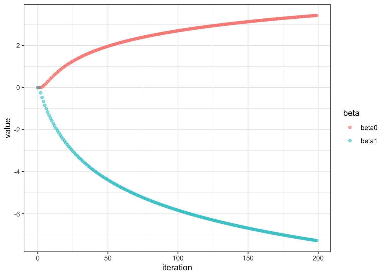
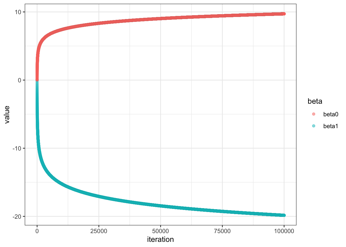
Very interesting. The plot shows non-convergence even after 200 iters. Let’s see what it looks like after max iteration of 100000
Let’s visualize our gradients of the first 200 iters
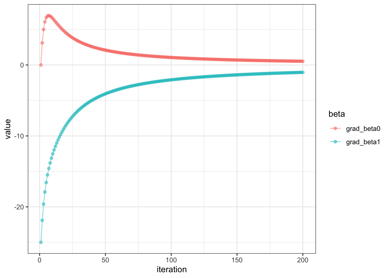
Looks quite odd indeed!
Let’s compare it with glm again
glm_model <- glm(y ~ x, family = binomial())
summary(glm_model)
##
## Call:
## glm(formula = y ~ x, family = binomial())
##
## Coefficients:
##             Estimate Std. Error z value Pr(>|z|)
## (Intercept)    26.57   50363.44   0.001    1.000
## x             -53.13   71224.73  -0.001    0.999
##
## (Dispersion parameter for binomial family taken to be 1)
##
##     Null deviance: 1.3863e+02  on 99  degrees of freedom
## Residual deviance: 5.8016e-10  on 98  degrees of freedom
## AIC: 4
##
## Number of Fisher Scoring iterations: 25
Wow, quite similar results !!! Interesting note to myself, if we use x <- seq(1,100,1) instead of binary, for optim our SE won’t be as big, it’s qctually soooo much smaller than glm. Maybe because of the optimization method used, since glm uses IWLS if I’m not mistaken.
Final Thoughts
- Wow, trying to figure out some of these fundamentals are really refreshing!
- It makes calculating MLE for other GLM much easier!
- We got to practice our calculus, which is quite cool! Lots of tries! Lots of errors!
- If we face complete separation from real data, here are some possible solutions
- Striving to be perfect is not a natural thing for the language of the universe
Addendum:
Click here to go to the next post on using Fisher information Iteration & how we used the entire information matrix (hessian) to derive Netwon-Raphson method.
Lessons Learnt
- A complete separation in logistic regression, symptoms are non-convergence, extreme estimates, and large standard errors, very small residual deviance
- learnt maximum likelihood estimation for logistic regression
- practiced calculus, refreshed on chain rule, quotient rule, matrix inverse
- learnt how to use
optim - learnt about Hessian matrix and Fisher information
- learnt about Cramér-Rao Lower Bound (CRLB) and its significance in MLE
- for some reason
\\does not work as well as\\\or\newlinein latex when convertrmdtomd
If you like this article:
- please feel free to send me a comment or visit my other blogs
- please feel free to follow me on BlueSky, twitter, GitHub or Mastodon
- if you would like collaborate please feel free to contact me
- Posted on:
- May 17, 2025
- Length:
- 16 minute read, 3274 words
- Categories:
- r R hessian maximum likelihood estimation derivative chain rule quotient rule optim mle complete separation