Assessing TEM, CTX-M, and KPC-2 With Molecular Docking and Molecular Dynamic Simulation

🧬 Testing beta-lactamase resistance with AlphaFold + DiffDock + GROMACS! Watch clavulanic acid bind TEM-5, CTX-M-15, KPC-2, and get rejected by TEM-30. Simulation confirms biology! 🔬💊

Motivations

Now that we’ve learnt the pipeline of molecular docking and molecular dynamic simulation. Let’s check some of the other proteins and ligand and see if these make sense. Let’s assess ESBL beta lactamase since we did something before ( here). Let’s check some of the hypothesis here, some TEMs are inhibitor resistant such as TEM-30, whereas ESBL beta lactamases like TEM-5 and CTX-M-15 can be susceptible to beta lactamase inhibitor such as clavulanic acid, whereas TEM-30, we should see that it won’t bind. We’ll also assess KPC2, which is a carbapanemase, it does bind to clavulanic acid, however, instead of being an inhibtor, it actually hydrolyzes it. But let’s see what MD results we get!

This time, we will get protein sequence of interest and use AlphaFold Server to predict our protein and generate pdb, and instead of relying on known coordinates of the protein, let’s use DiffDock to screen the best docking site, then use that for MD simulation. We will write some instructions on DiffDock, how to install and run it. But we will leave off the MD simulation part, we can refer to here. But I will run a good chunk of code to assess our results so that at least I don’t have to copy and paste multiple times to assess RMSD, RMSF, hydrogen bonds, gyration, and distance. We will also have some cool visuals! Let’s test this out!

Objectives:

• Get Our Proteins
• Protein Prediction With AlphaFold
• Using DiffDock to predict binding sites
• Assess Results
  • TEM-5
  • CTX-M-15
  • TEM-30
• Opportunities for improvement
• Lessons Learnt

Get Our Proteins

We go here and select the gene of interest and go to Refseq.

Then click on Fasta which will bring us to this.

Copy the protein sequence and we’ll move on to our next step. Also don’t forget to copy the other proteins of interest, in our case TEM-30, CTX-M-15, and KPC2.

Protein Prediction With AlphaFold

We will then visit Alphafold Server, you will have to login and then enter the sequence, and continue. Make sure to rename it to something you can recognize. Let it run, will likely take a minute. Then download it. Unzip it and you will see 5 cif files. I usually use the first one which ends with 0.

Using DiffDock to predict binding sites

Install

git clone https://github.com/gcorso/DiffDock.git
conda env create --file environment.yml
conda activate diffdock

You can check the github link out. From my experience, the above worked on Ubuntu but failed on my mac. I actually had to use Claude Code to help me install it. Could be just a me thing.

Let’s take a look at this protein with ChimeraX.

Do you see the big protein with a long tail? The long tail has low prediction score and is likely to be disordered, so we will remove that part and just keep the globular part. We can do that with ChimeraX, just select the tail and delete it. Then save it as a new pdb file.

Then we will run DiffDock to predict the binding site. We will use clavulanic acid as our ligand. You can download it from PubChem. Then we will run DiffDock with the following command:ea, we should be very careful not to use it.

obabel alphafold0.cif -O tem5.pdb

# make sure you're in DiffDock folder and has activate your conda env that used to install
python3 inference.py \
  --protein_path tem5.pdb \
  --ligand "OC(=O)[C@@H]2/C=C\1OC[C@@H](O)/C1=C\N2" \ 
  --out_dir results_tem5_step20 \
  --inference_steps 20 \
  --samples_per_complex 10 \
  --batch_size 5
  
# create ligand pdb
obabel rank1.sdf -O clav_acid.pdb

You see the ligand SMILES? 😀 We don’t need to download one from pubchem. You can just copy the SMILES from it. Woo hoo! Once you ran the above it will have 10 ranks. Open (with ChimeraX) the protein pdb first and then all the rank docked positions to visually assess the predicted docking sites.

Alright, it looks like there is one pocket (including the top 1 ranked position) is in that one pocket that in the middle of the picture.

If you take a look at the files produced by DiffDock, it ranks its confidence score at the end of the file, the lower the better.

Alright, go through the MD simulation procedure, wait and assess!

Note: I found that I could use 2 GTX 1080 and run each GPU with one protein-ligand interaction, and also use && and chain multiple mdrun commands so that it can go from one simulation to another after it’s done! For example gmx mdrun blab blah && cd /path/to/another && gmx mdrun blah blah. Also, make sure to use tmux when you’re running the production.

Assess Results

echo -e "\"Protein\" | \"UNL\"\nq" | gmx make_ndx -f md.gro -o index.ndx
echo "0" | gmx trjconv -s md.tpr -f md.xtc -o md_nojump.xtc -pbc nojump
echo "Protein_UNL System" | gmx trjconv -s md.tpr -f md_nojump.xtc -o md_noPBC.xtc -pbc mol -center -n index.ndx
echo '4 13' | gmx rms -s md.tpr -f md_noPBC.xtc -o rmsd_ligand.xvg -tu ns -n index.ndx
echo '4 4' | gmx rms -s md.tpr -f md_noPBC.xtc -o rmsd_protein.xvg -tu ns -n index.ndx
echo 4 | gmx rmsf -s md.tpr -f md_noPBC.xtc -o rmsf_protein.xvg -res 
echo 13 | gmx rmsf -s md.tpr -f md_noPBC.xtc -o rmsf_ligand.xvg 
echo '1' | gmx gyrate -s md.tpr -f md_noPBC.xtc -o gyrate.xvg 
echo '1 13' | gmx hbond -s md.tpr -f md_noPBC.xtc -num hbond_ligand_protein.xvg -tu ns 
echo '1 13' | gmx mindist -f md_noPBC.xtc -s md.tpr -od mindist_prot_lig.xvg -on numcont_prot_lig.xvg -d 0.4
gmx distance -f md_noPBC.xtc -s md.tpr -select 'com of group "Protein" plus com of group "UNL"' -oall distance_prot_lig.xvg
if grep -q "^;energygrps" md.mdp; then
    sed -i 's/^;energygrps/energygrps/' md.mdp
    echo "Uncommented energygrps"
elif grep -q "^energygrps" md.mdp; then
    echo "energygrps already active, doing nothing"
else
    echo "energygrps = Protein UNL" >> md.mdp
    echo "Added energygrps"
fi
gmx grompp -f md.mdp -c md.gro -p topol.top -o rerun.tpr 
gmx mdrun -s rerun.tpr -rerun md_nojump.xtc -e rerun.edr -ntmpi 1 -ntomp 4 
printf "Coul-SR:Protein-UNL\nLJ-SR:Protein-UNL\n0\n" | gmx energy -f rerun.edr -o interaction_energy.xvg
cp *.xvg /path/to/your/analysis

Note: Make sure to run the above after we’re done with all of the simulation, otherwise it will bottleneck both. Meaning, it will be slow for the above and also your active simulation. Well, I only have 4 core, so it might be different for yours! It might not matter at all. Above I would use -ntomp 2 if my other simulation is still running but i want to check the result.

Create function to visualize all

library(tidyverse)
library(xvm)
library(ggpubr)

plot_all <- function(path,int=T) {
prot <- read_xvg(paste0(path,"rmsd_protein.xvg"))
ligand <- read_xvg(paste0(path,"rmsd_ligand.xvg"))
rmsf_prot <- read_xvg(paste0(path,"rmsf_protein.xvg"))
rmsf_ligand <- read_xvg(paste0(path,"rmsf_ligand.xvg"))
gy <- read_xvg(paste0(path,"gyrate.xvg")) 
if (int) {
interaction <- read_xvg(paste0(path,"interaction_energy.xvg"))
plot_interaction <- plot_xvg(interaction)}
hbond <- read_xvg(paste0(path,"hbond_ligand_protein.xvg"))
mindist <- read_lines(paste0(path,"mindist_prot_lig.xvg"))
dist <- read_lines(paste0(path,"distance_prot_lig.xvg"))

plot_rmsd_prot <- plot_xvg(prot)
plot_rmsd_ligand <- plot_xvg(ligand)
plot_rmsf_prot <- plot_xvg(rmsf_prot)
plot_rmsf_ligand <- plot_xvg(rmsf_ligand)
plot_gy <- plot_xvg(gy)
plot_hbond <- tibble(hbond$hbond_ligand_protein.xvg$data) |> 
  distinct() |>
 ggplot(aes(x=`Time (ns)`,y=`Hydrogen bonds`)) +
 geom_line(color = "red", alpha=0.8) +
 theme_bw() +
  ggtitle("Hydrogen bonds")

mindist_list <- mindist[!str_detect(mindist, "^@|^#")] |> str_split(" ")
time <- mindist_val <- vector(mode = "numeric", length = length(mindist_list))
for (i in 1:length(mindist_list)) {
  time[i] <- mindist_list[[i]][1]
  mindist_val[i] <- mindist_list[[i]][3]
}

mindist_df <- tibble(time = time, mindist_val = mindist_val) |>
  mutate(time = as.numeric(time),
         mindist_val = as.numeric(mindist_val))

plot_mindist <- mindist_df |>
  ggplot(aes(x=time,y=mindist_val)) +
  geom_point(color = "red", alpha=0.7) +
  theme_bw() +
  ggtitle("Min Distance")


dist_list <- dist[!str_detect(dist, "^@|^#")] |> str_trim() |> str_split("    ")

time <- dist_val <- vector(mode = "numeric", length = length(dist_list))
for (i in 1:length(dist_list)) {
  time[i] <- dist_list[[i]][1] 
  dist_val[i] <- dist_list[[i]][2]
}

dist_df <- tibble(time = time, dist_val = dist_val) |>
  mutate(time = as.numeric(time),
         dist_val = as.numeric(dist_val))

plot_dist <- dist_df |>
  ggplot(aes(x=time,y=dist_val)) +
  geom_point(color = "red", alpha=0.7) +
  theme_bw() +
  ggtitle("Distance Between Protein and Ligand")

if (int) {
plotlist <- list(plot_rmsd_prot, plot_rmsd_ligand, plot_rmsf_prot, plot_rmsf_ligand,
                 plot_gy, plot_interaction, plot_hbond, plot_mindist, plot_dist) }
else {plotlist <- list(plot_rmsd_prot, plot_rmsd_ligand, plot_rmsf_prot, plot_rmsf_ligand,
                 plot_gy, plot_hbond, plot_mindist, plot_dist)}
return(ggarrange(plotlist = plotlist, ncol = 2))
}

TEM-5

plot_all("tem5_result/")

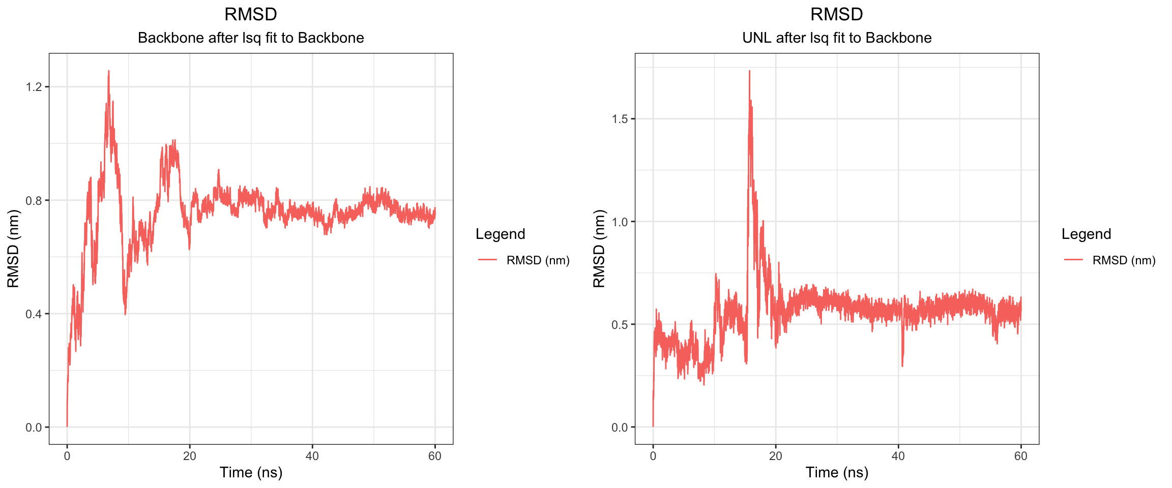
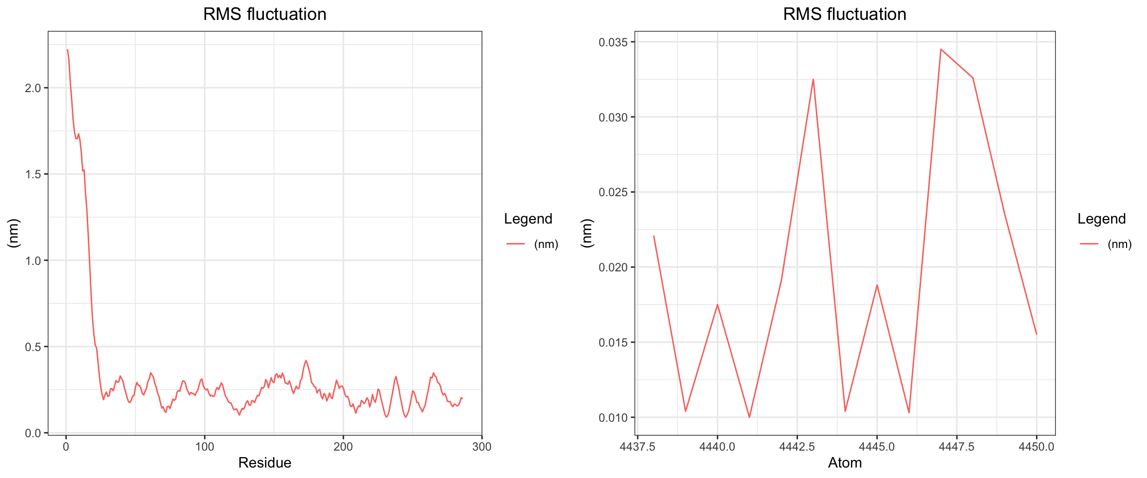
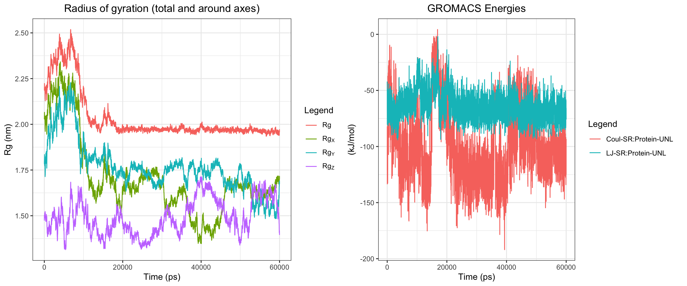
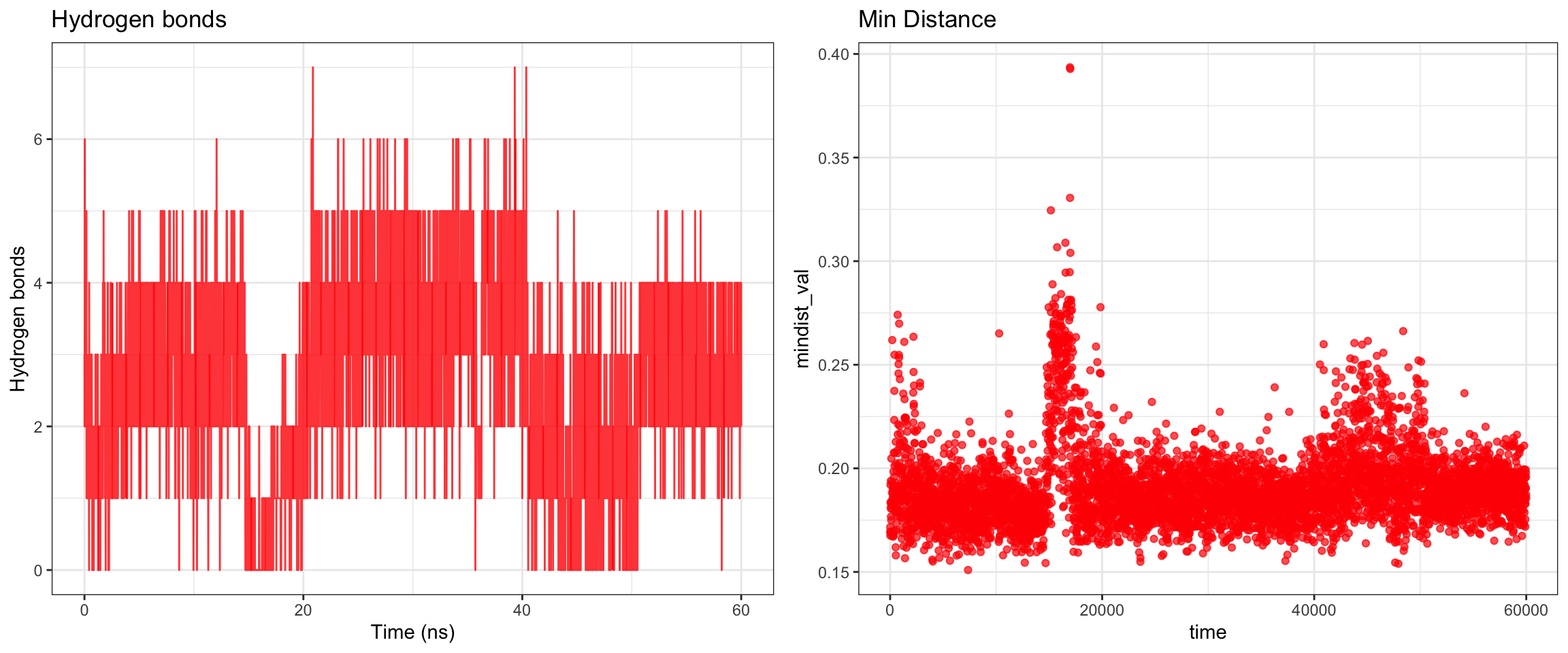
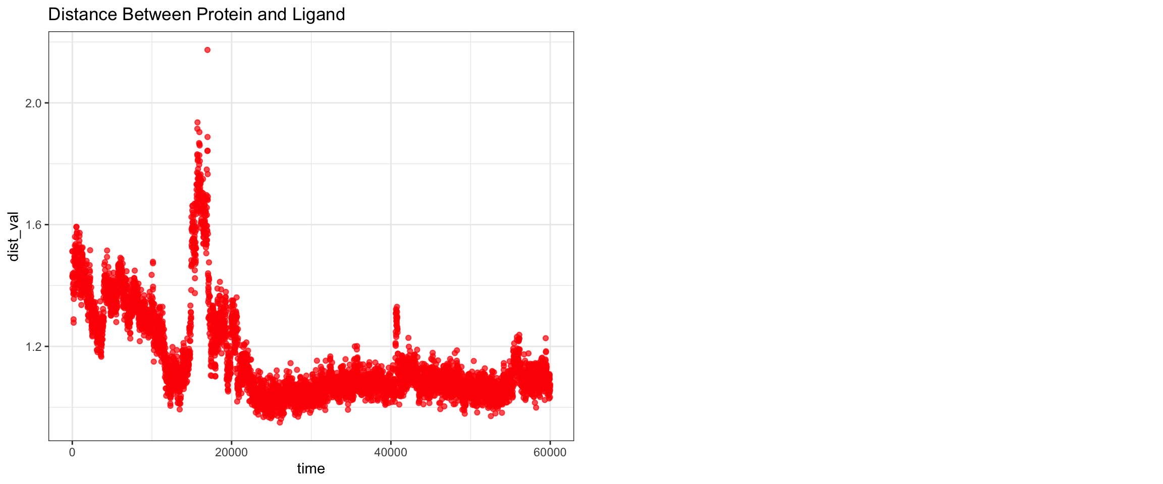
Overall, clavulanic acid and TEM-5 demonstrated stable binding throughout the 60 ns simulation. The protein RMSD plateaued early, confirming stable conformation, ligand rmsf has also plateaud. The total radius of gyration remained largely stable, and both Coulombic and Lennard-Jones interaction energies stayed consistently negative, indicating favorable protein–ligand interactions. Hydrogen bonds were maintained at around 2–4 throughout the simulation, which is adequate for a small molecule ligand. Both the center-of-mass and minimum distances converged to stable low values and remained consistent for the remainder of the trajectory. Collectively, these results support a successful molecular dynamics simulation with stable ligand binding.

CTX-M-15

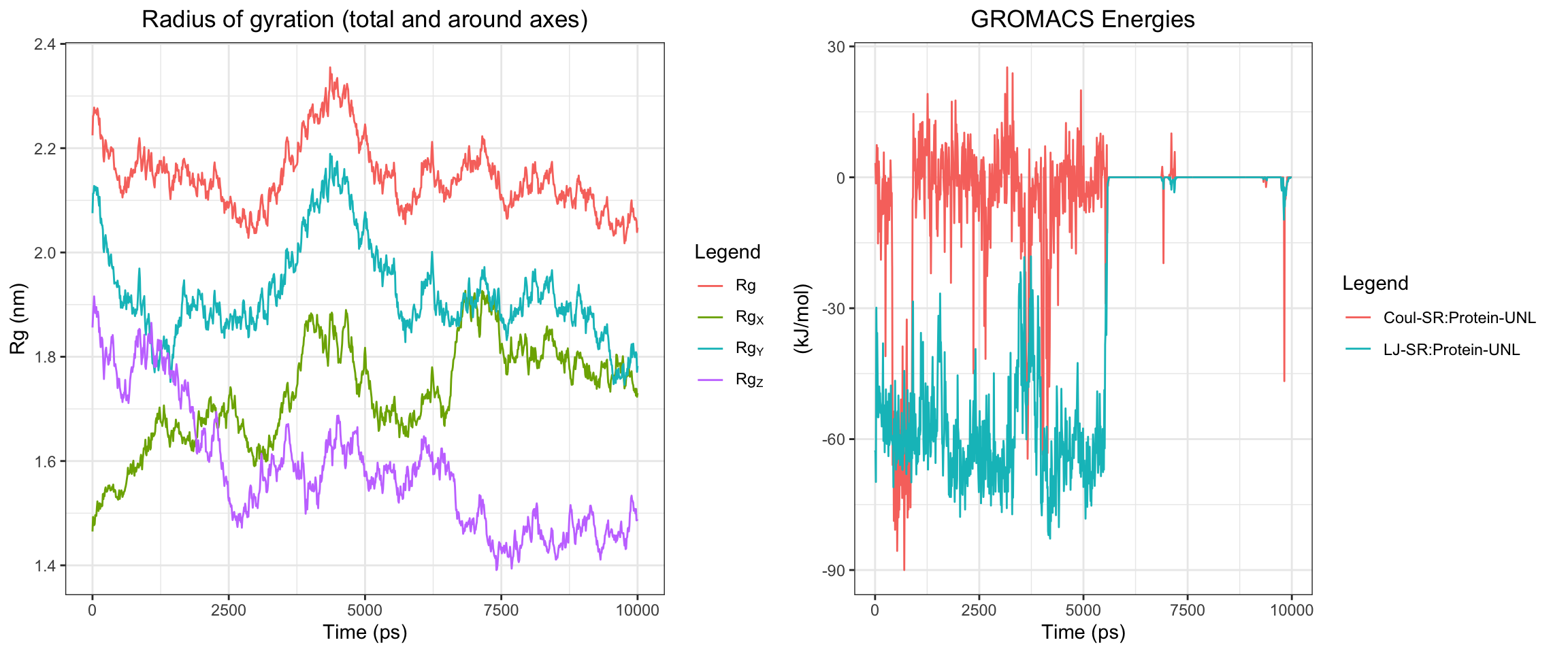
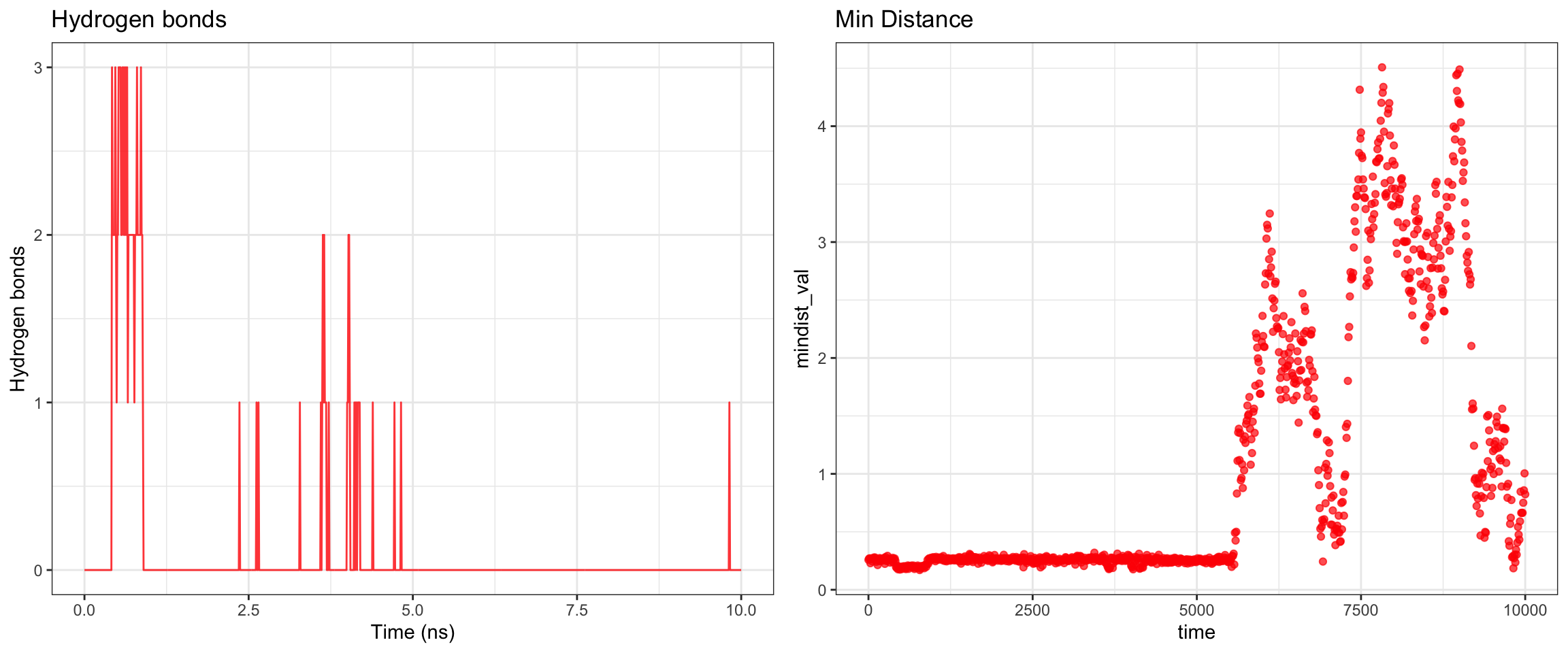
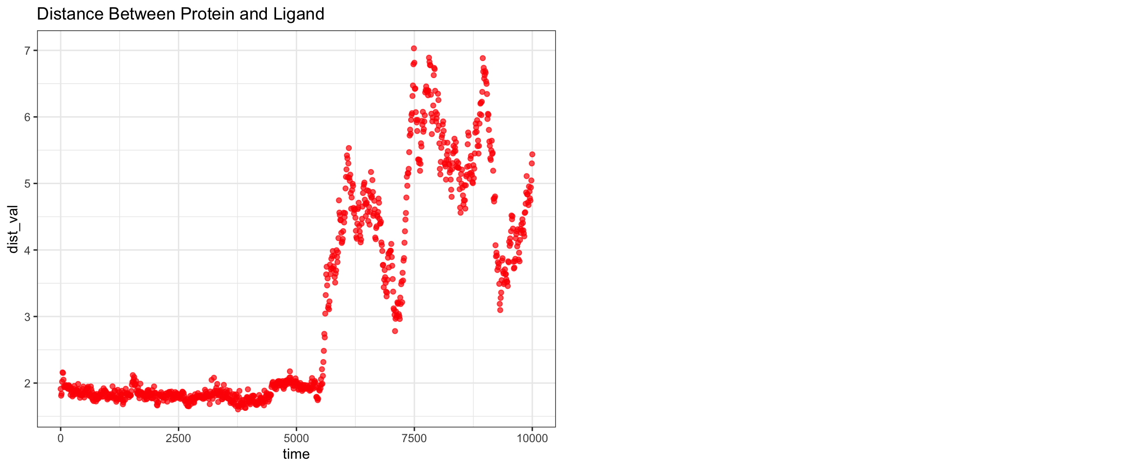
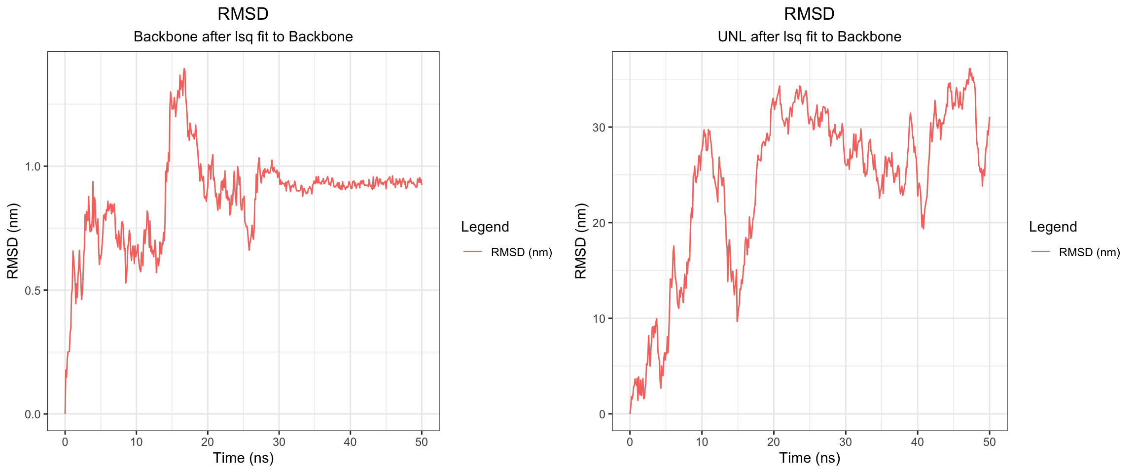
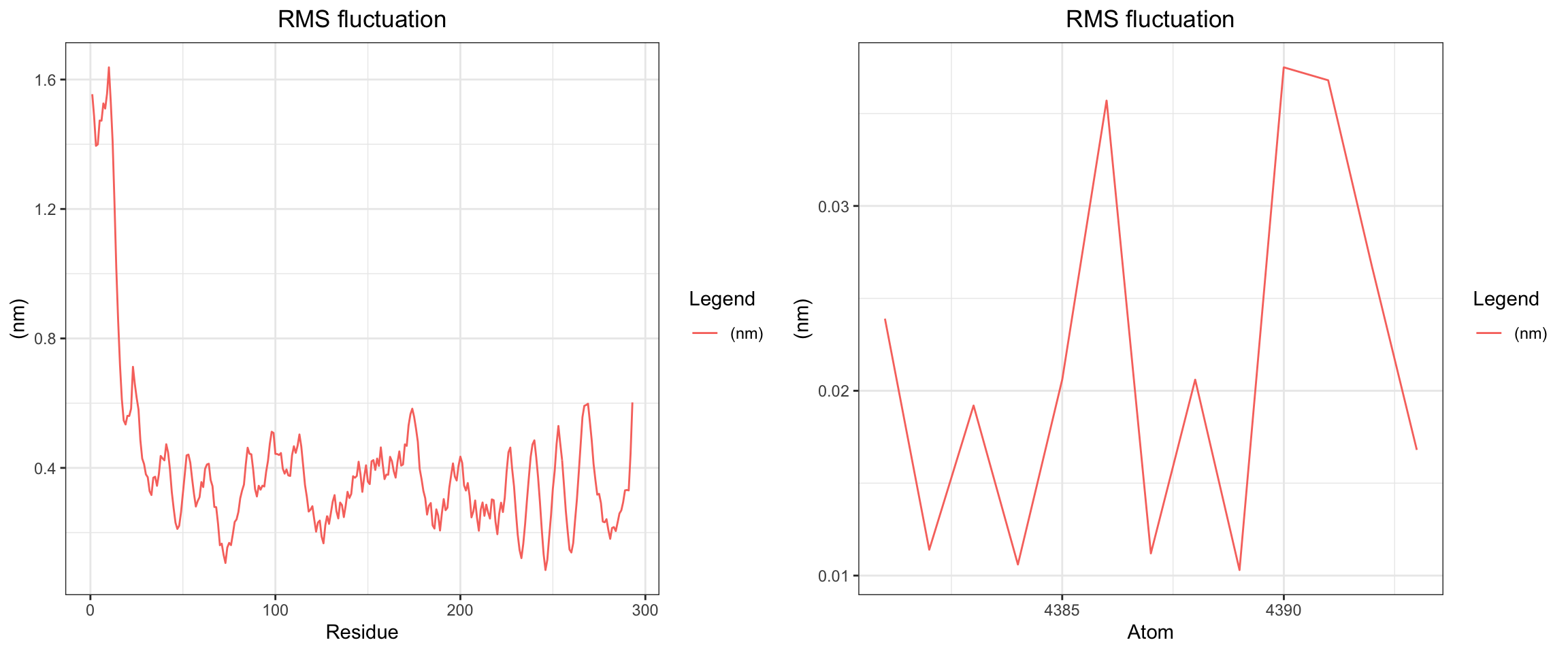
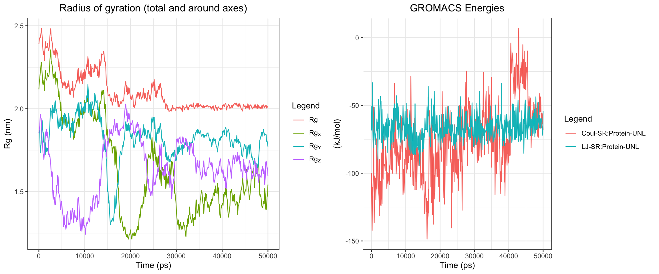
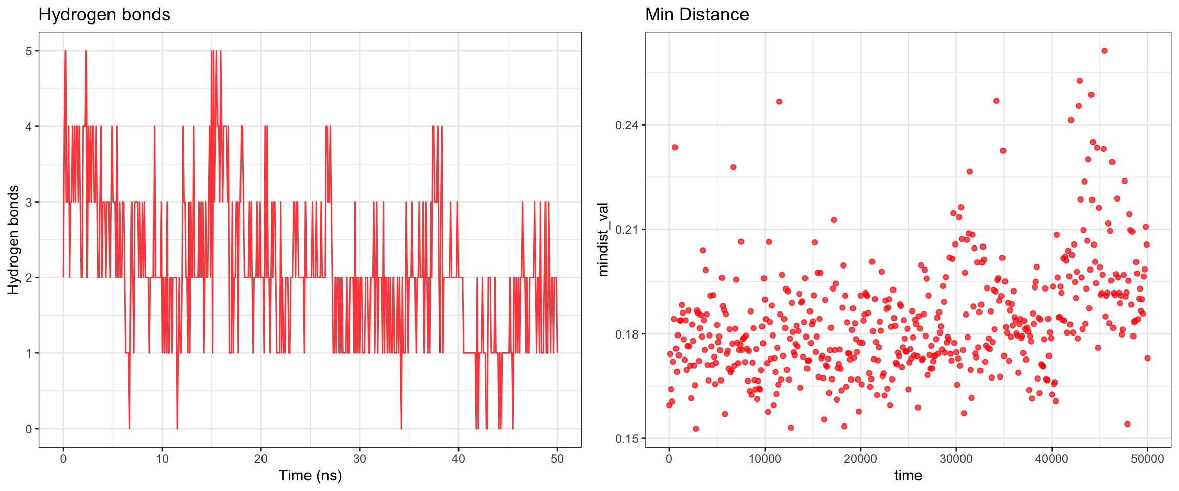
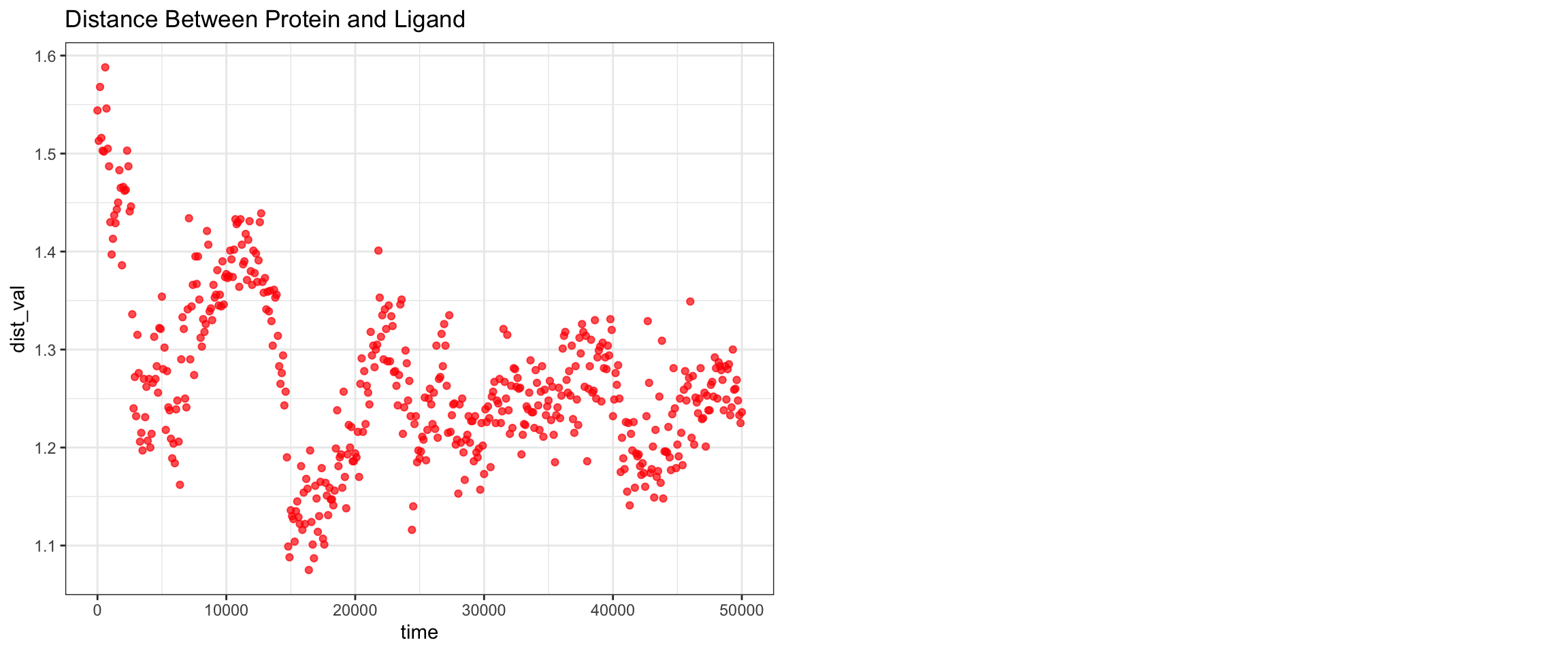
plot_all("ctxm15_result/")

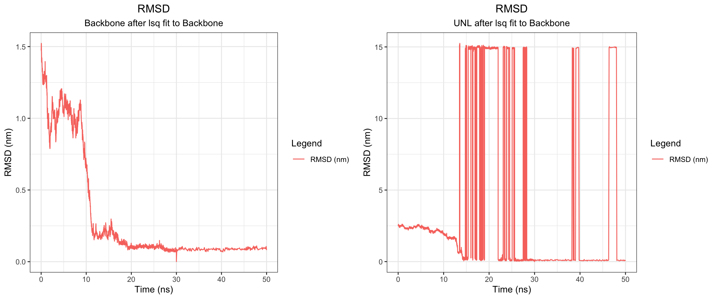
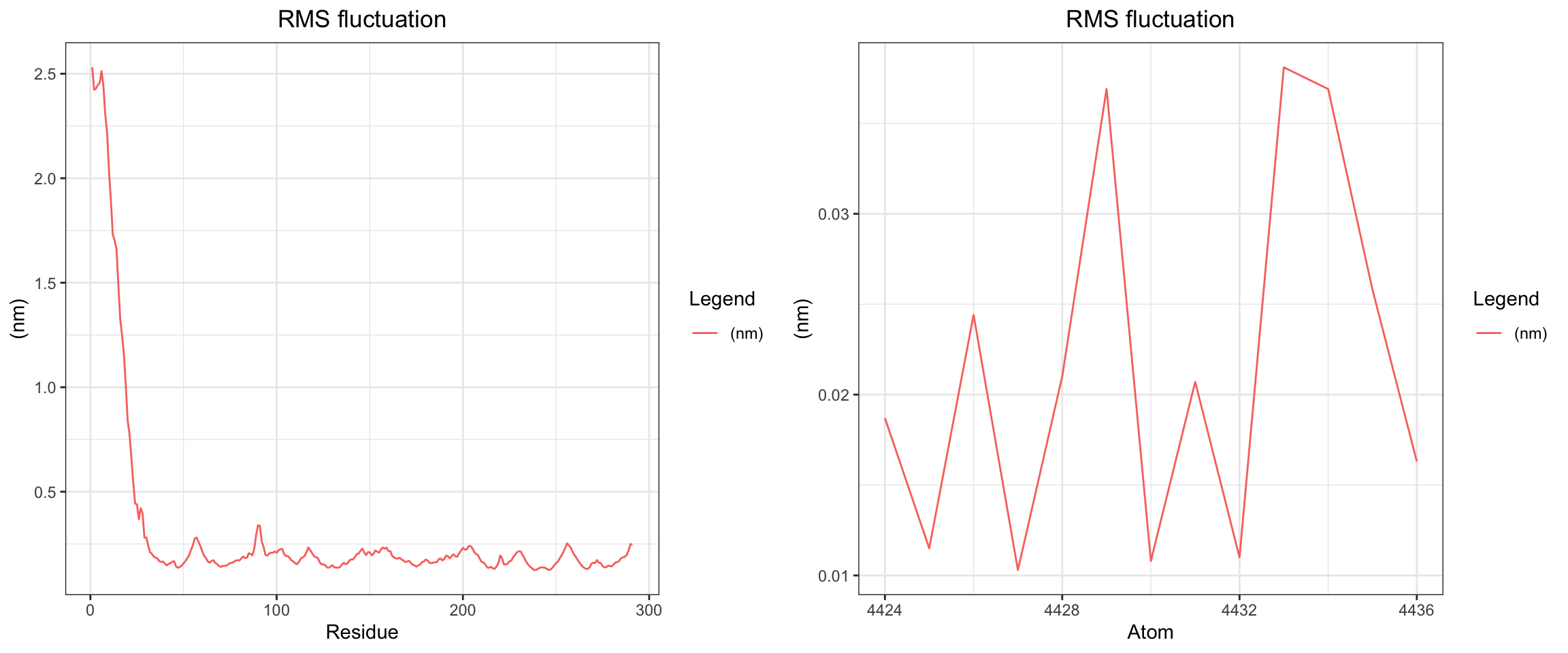
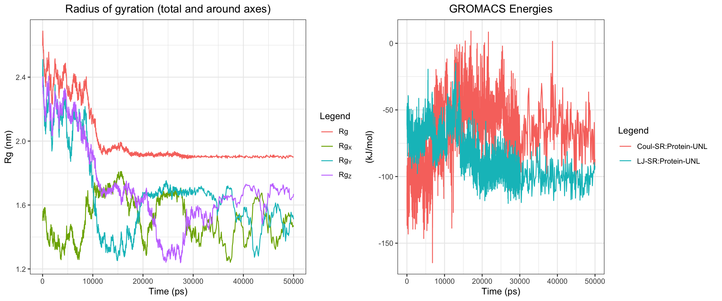
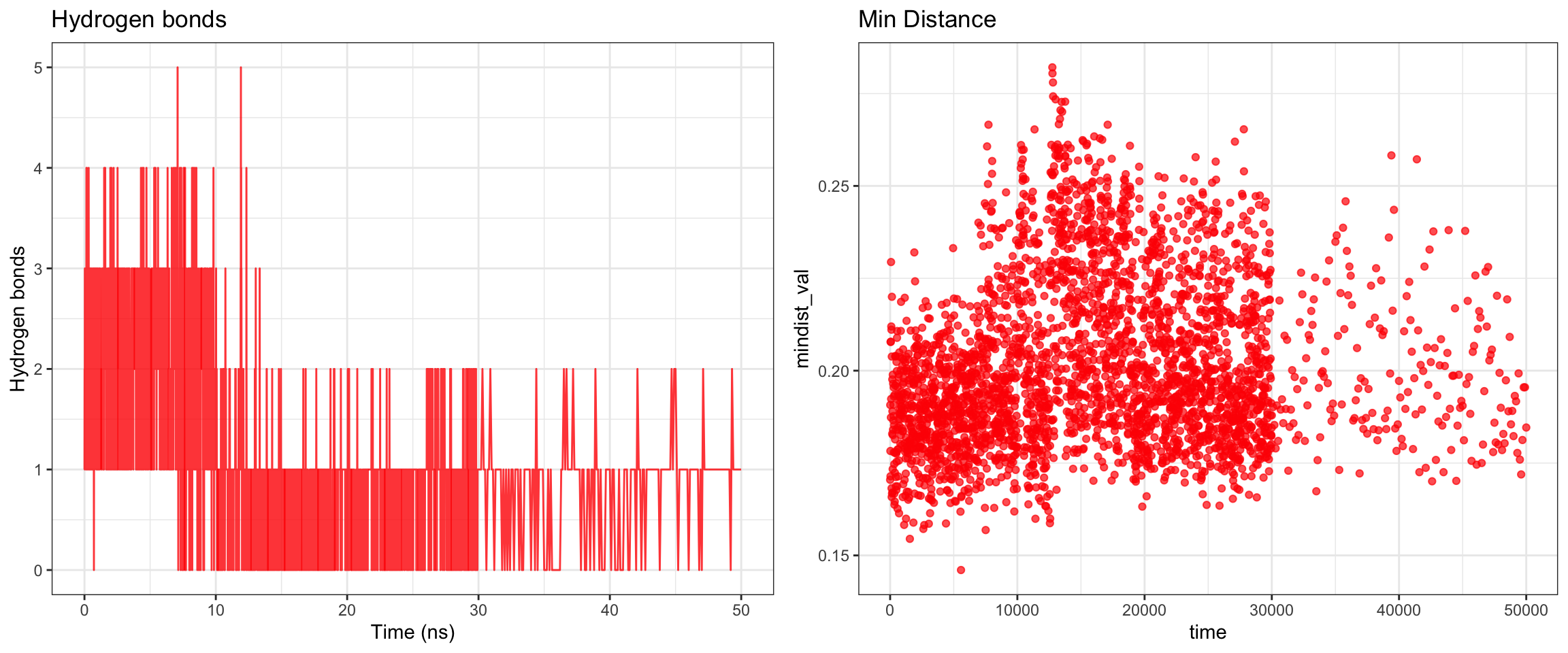
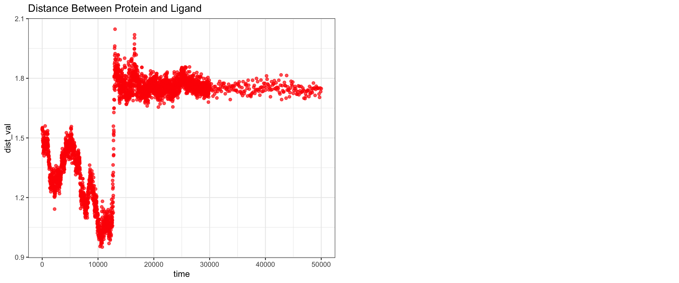
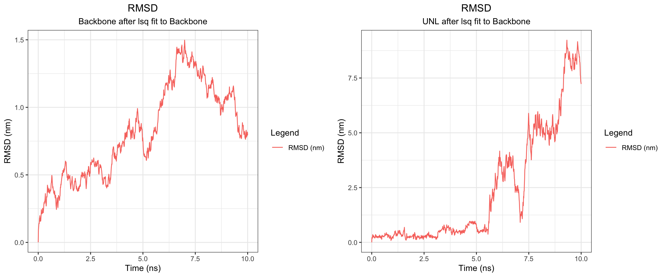
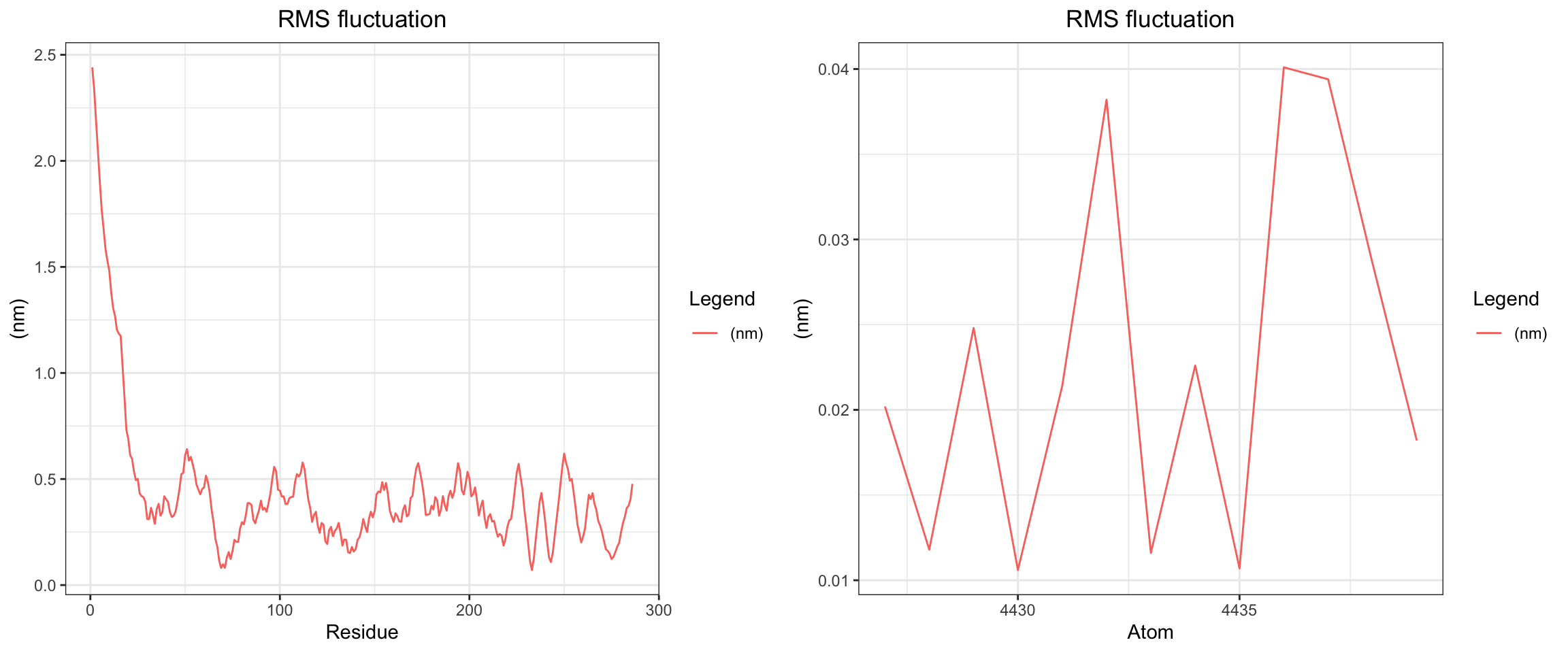
Overall, clavulanic acid and CTX-M-15 also demonstrated stable binding throughout the 50 ns simulation. Although the ligand RMSD shows significant noise — likely due to improper initial coordinate assignment when using the ACPYPE-generated .gro file instead of the docked ligand coordinates — the protein RMSD plateaued and remained stable. This is not a sign of dissociation as a true dissociation ( see here) would look like this. The total radius of gyration was similarly stable. Interaction energies and hydrogen bond counts were consistent throughout the trajectory, indicating sustained non-covalent interactions. Both the minimum distance and center-of-mass distance between the protein and ligand converged and remained low, further supporting stable binding. Also, upon visualizing the md.xtc in reference to the first frame of pdb, we can see there was at one point the ligand may have dissociated at a short period of time and then reattached.

TEM-30

plot_all("tem30_result/")

This simulation presents a clear case of true ligand dissociation, indicating that clavulanic acid does not bind well to TEM-30. Notably, the simulation terminated early. Both the protein and ligand RMSD rose continuously without plateauing, though the protein RMSD values may be inflated due to the same coordinate assignment error noted previously. More definitively, both hydrogen bond counts and interaction energies dropped to zero, and the minimum distance as well as the center-of-mass distance between the protein and ligand diverged progressively over time. Collectively, these findings confirm that stable binding was not achieved in this simulation. Below, you can see ligand flies away from the pocket site.

KPC2

plot_all("kpc2_result/")

Finally, the KPC-2 and clavulanic acid simulation also demonstrated stable binding throughout the 50 ns trajectory. As noted previously, the ligand RMSD cannot be accurately interpreted due to the coordinate assignment error. Nevertheless, both interaction energies and hydrogen bond counts remained consistent throughout, and the minimum distance as well as the center-of-mass distance between the protein and ligand converged to lower values and remained stable. Importantly, however, stable binding in this simulation does not imply that clavulanic acid acts as an inhibitor of KPC-2. In fact, KPC-2 is known to hydrolyze clavulanic acid — a covalent enzymatic process that a non-covalent molecular dynamics simulation such as this cannot capture or reflect.

Final Thought

Wow, having the previous workflow really helps with lower the risk of error! I definitely learnt that my mistake of using acpype coordinates have caused significant noise on rmsd ligand and should really use the docked ligand position to create the complex.gro. Still so much to learn! But this is a really cool simulation where we can test the tested hypothesis and see it with our own eyes! I’m so grateful and fortunate to be able to be at this time period to learn these without TOO much disappointments. And also so grateful for all these scientists to be able to share these techniques for free! That is truly amazing and inspiring! ❤️

Opportunities for improvement

• I have been mistakenly using acpype gro coordinates to make complex.gro, where the rmsd ligand was way off but everything else seem to be fine. We should be using the docked pose to convert to gro using gmx editconf -f diffdock_pose.pdb -o ligand_positioned.gro
• Learn how to find out if there is consistent non-covalent bond between ligand and protein, how do we then differentiate between the ligand inactivating the protein or that the protein hydrolyzes the ligand like KPC2
• Learn how to perform covalent docking and covalent md simulation
• rewrite md sim pipeline into something easier to automate. currently i have to copy and paste from my previous documentation, mind you it’s already REALLY helpful because i was able to do all those in the matter of minutes. Let’s see how we can further optimize that, more ergnomics.
• Try colabfold locally to produce protein, might take some time

Lessons Learnt

• I did not know that CTX-M-15 can bind to clavulanic acid, did the simulation first then realized it bound and verified literature and apparently it does! Simulation is another tool to help to learn something new!
• I change the output md.mdp to 50000 instead of 5000 to reduce bottle neck between cpu and gpu
• use && chaining to run one production after another
• can independently use 2 or more GPU if motherboard allows
• gromacs automatically chooses a GPU that has better capacity and assign that as 0?
• need to center in order for a good visualization, otherwise you will see protein and ligand might split as it exits the edge of simulation box, it enters from the other end.

If you like this article:

• please feel free to send me a comment or visit my other blogs
• please feel free to follow me on BlueSky, twitter, GitHub or Mastodon
• if you would like collaborate please feel free to contact me