Exploring Molecular Docking & Molecular Dynamic Simulations - A Note To Myself

🧬 Explored molecular docking & MD simulations with penicillin binding to PBP2x — lots of stumbling through GROMACS but slowly piecing it together! 💊 Still much more to learn, but we’re getting there! 🔬

Motivations:

Since last year I’ve been fascinated by how scientists are able to use computational methods and simulation of the physical world. Things such as moelcular dynamic is quite amazing! And we can learn by running through these processes. Since we know that penicillin binds to penicillin binding protein 2x, why don’t we use that as a stepping stone and see how far we can go? Oh, have you used Claude Code or OpenAI Codex? If not, these are great tools to maybe get to the end first and see the results and then document and learn step by step from 0 to n to get to that final result? I found that extremely helpful because I know that if this works, it should work by going through the steps again and there is light at the end of the tunnel! Also, not to mention, these tools as they’re getting to the end, will let you know if your machine is not powerful enough to get there 🤣 Now, buckle up! This is REALLY going to be bumpy. All codes are in bash. We’ll set a pipeline with either python or R in the future for more experiments!

Just so happen, today is Valentine’s Day. Happy Valentine’s Day! ❤️ Molecular docking and simulation is like a match making activity 🤣 What a coincidence!

Disclaimer:

I am not a biochemist. This blog serves as a note for reproducibility for my own and only for educational purposes and documentation of what worked and what didn’t, so that I won’t repeat the same mistake in the future. If you noticed any error, please educate me! Also, most codes below are run in Ubuntu bash, some in R for visualization. Also I used a lot of Claude to help discover, debug, learn.

Objectives:

• What is Molecular Docking & Molecular Dynamic Simulations?
• Molecular Docking
  • Autodock Vina Installation
  • Download
  • Convert Protein and Ligand Structures
  • Run Vina
• Molecular Dynamic Simulation
  • Gromacs Installations
  • Prepare Protein
  • Prepare Ligand
  • Create Position Restraints For The Ligand
  • Edit topol.top
  • Create The Complex
  • Definte Simulation Box
  • Create Solvent
  • Add Ion
  • Energy Minimization
  • NVT Equilibration
  • NPT Equilibration
  • Production
• Asessment
  • RMSD
  • RMSF
  • Radisu of Gyration
  • Interaction
  • H bond
  • Binding Distance
  • Visual Inspection
• Opportunities for Improvement
• Lessons learnt

Please take a look at this Gromacs Tutorials, has a lot o fanstastic code to help beginners like me!

What Is Molecular Docking & Molecular Dynamic Simulations?

Molecular docking is basically computational lock and key exploration - you’re predicting how a small molecule (like a medicine) will bind to a protein target by testing different orientations and conformations to find the lowest energy binding pose. It’s a static snapshot: protein and ligand are treated as relatively rigid (or semi-flexible), and you get binding scores that estimate affinity. Molecular dynamics (MD) simulation takes it way further - it’s like watching a molecular movie where you simulate the actual physics of atoms moving over time (picoseconds to microseconds), accounting for solvent, temperature, and all the wiggling and conformational changes that happen in real biological systems. Docking gives you the “where and how tight,” while MD gives you the “what happens next” - stability, induced fit, binding pathways, and whether that docked pose actually holds up when everything’s allowed to move realistically. You often use docking first to generate binding hypotheses, then validate or refine them with MD.

Molecular Docking

Installation

sudo apt update
sudo apt install autodock-vina # I have version `1.2.5`. 
sudo apt install openbabel # I have version 3.1.0

Download

Now, we have to download ligand and protein structures. Let’s go to RCSB and download our protein.

We’ll be working with Penicillin-binding Protein 2x.

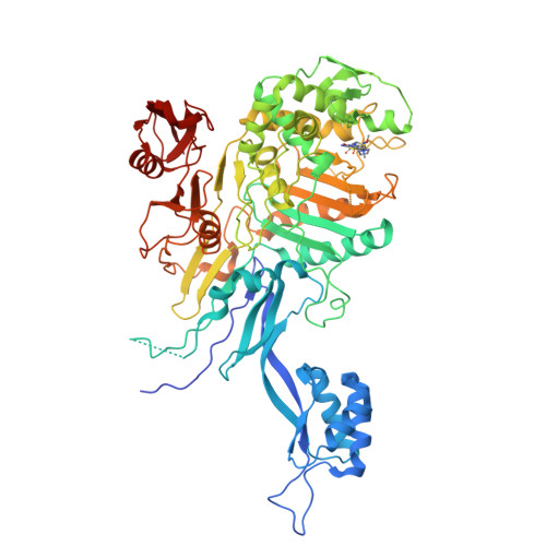
This one is from Streptococcus pneumoniae with cefepime already bound to it. So at least we know where is the binding site and we can estimate using the coordinates on our penicillin.

Download the pdb. If we use ChimeraX to visualize the pdb, it will look something like this. With the ligand (cefepime) highlighted in green.

If we simply just read the pdb file of what we just downloaded, as you scroll through you will see ATOM means standard protein/nucleic acid atoms and HETATM = heteroatoms like ligands, waters or ions.

In the middle where we see lots of columns of numbers, the xyz coordinates of where ligand (cefepime aka 9WT) is located on this protein. We will use this coordinate to set up our docking later on. Take note that in the middle where we see lots of columns of numbers, the xyz coordinates of where ligand (cefepime aka 9WT) is located on this protein. The coordinates are around x=30, y=-15, z=50. Remember this, because we will need this for docking.

Next we’ll download a penicillin G where we will go to PubChem instead.

Convert Protein and Ligand Structures

This is not always the case, but because of our protein already contains a ligand, let’s remove that ligand and createa clean pbp2x_protein.pdb then pdbqt which is the format that vina uses.

# remove ligand from protein pdb
grep "^ATOM" 5OJ0.pdb > pbp2x_protein.pdb

# convert pdb and sif files to pdbqt for autodock
obabel pbp2x_protein.pdb -O pbp2x_protein.pdbqt -xr #(-xr removes non-polar hydrogens)
obabel Conformer3D_COMPOUND_CID_5904.sdf -O pcn.pdbqt -xh #(-xh add hydrogen needed for proper docking)

Run Vina

vina --receptor pbp2x_protein.pdbqt --ligand pcn.pdbqt \
     --center_x 30.0 --center_y -15.0 --center_z 50.0 \
     --size_x 30.0 --size_y 30.0 --size_z 30.0 \
     --exhaustiveness 16 \
     --num_modes 1 \
     --out pcn_docked.pdbqt 

## turn pdbqt back to pdb
obabel pcn_docked.pdbqt -O pcn_docked.pdb

--num_nodes will only show the top 1 predicted pose and turn it into pcn_docked.pdbqt. We will convert this back to pdb for visualization and later use in molecular dynamic simulations.

After it’s done. It will look something like this. For more question and answer information please see this. It has a lot of answers, one of them is what is a good search size?

You should probably avoid search spaces bigger than 30 x 30 x 30 Angstrom, unless you also increase “–exhaustiveness”.

With affinity of -6.83 kcal/mol. Is this considered OK? From my shallow reading, the smaller the better. General < -7 is good (some said -10 arbitarily). If it’s > -5, it means it’s less likely to bind. So this is borderline, but we can still use it for molecular dynamic simulations to see if it holds up. But before that, let’s try an experiment, what if we dock a compound that we know doesn’t bind to this protein, say aspirin?

Alright! Pretty good! -4.968 is the predicted binding affinity of aspirin to our protein target. Much less than our penicillin! Ideally with virtual screening, we want to have a lot of ligands that we want to run through and find the top hits.

Molecular Dynamic Simulation

Install Gromacs

# Install dependencies
sudo apt update
sudo apt install -y build-essential cmake git libfftw3-dev libopenmpi-dev wget

# Install NVIDIA drivers and CUDA (if not already installed)
sudo apt install -y nvidia-driver-535 nvidia-cuda-toolkit

# Download GROMACS
cd ~
wget https://ftp.gromacs.org/gromacs/gromacs-2024.4.tar.gz
tar xfz gromacs-2024.4.tar.gz
cd gromacs-2024.4

# Build with GPU support
mkdir build
cd build
cmake .. -DGMX_BUILD_OWN_FFTW=ON -DGMX_GPU=CUDA -DCUDA_TOOLKIT_ROOT_DIR=/usr/lib/cuda -DREGRESSIONTEST_DOWNLOAD=ON
make -j$(nproc)
sudo make install

# Add GROMACS to PATH permanently
echo 'source /usr/local/gromacs/bin/GMXRC' >> ~/.bashrc
source ~/.bashrc

# Verify installation
gmx --version

# Test GPU detection
gmx detect

Prepare Protein For Gromac

gmx pdb2gmx -f pbp2x_protein.pdb -o pbp2x_processed.gro -water tip3p -ff amber99sb-ildn

What this does is that it converts your protein PDB file into a simulation-ready format by adding hydrogen atoms, applying the AMBER99SB-ILDN force field parameters, and selecting the TIP3P water model. It outputs a processed structure file pbp2x_processed.gro and a topology file topol.top that contains all the molecular interaction parameters needed for running molecular dynamics simulations.

Prepare Ligand

acpype -i pcn_docked.mol2 -n 0 -a gaff2 -c bcc

This will create a directory called pcn_docked.acpype. what acpype does is that it takes your ligand structure (in this case pcn_docked.pdb) and generates the necessary topology and coordinate files for GROMACS. It uses the Antechamber tool to assign atom types and partial charges based on the AMBER force field, and outputs files like pcn_docked_GMX.itp (topology) and pcn_docked_GMX.gro (coordinates) that can be directly included in your GROMACS simulations.

Create Position Restraints For The Ligand

echo 0 | gmx genrestr -f pcn_docked.acpype/pcn_docked_GMX.gro \
             -o posre_ligand.itp \
             -fc 1000 1000 1000
             
## echo 0 means select "system"

Why do we need to do this? Because we want to make sure that our ligand doesn’t fly away during the equilibration phase. By creating a position restraint file for the ligand, we’re essentially telling GROMACS to apply a strong force (1000 kJ/mol/nm) to keep the ligand in place while the rest of the system (protein, water, ions) relaxes around it. This is especially important if we want to see how well our docked pose holds up under more realistic conditions without it drifting away from the binding site. I will use this ⛓️‍💥 to remind us where it is applied

Edit topol.top

By now you should have topol.top file. Open it and scroll down to

; Include Position restraint file
#ifdef POSRES
#include "posre.itp"
#endif

then add these chunk after it

; Include ligand position restraint file
#ifdef POSRES_LIGAND
#include "posre_ligand.itp"    ; remember this ⛓️‍💥 ?
#endif

Do you remember posre_ligand.itp that we created here ? We want to include this in topol.top so that when we’re at the phase of NVT and NPT, it will call this file to apply the restraint. We’re not done yet! More editing! Scary, right? I know.

After this, include these on your topol.top file as well.

#include "amber99sb-ildn.ff/forcefield.itp"
#include "pcn_docked.acpype/pcn_docked_GMX.itp"  ; Include ligand topology

[ system ]
Protein-Ligand Complex

[ molecules ]
Protein_chain_A    1
pcn_docked                1  ; Your ligand name from pcn_docked_GMX.itp

Take note that in [molecules] you have to insert your specific ligand name in your .itp file made from acpype.

Create The Complex

I’ve written myself a little cheat to do this by code

python3 << 'PYEOF'
   # Combine protein and ligand GRO files into complex.gro                      
                                         
   protein = "/your/path/pbp_test/pbp2x_processed.gro"
   ligand = "/your/path/pbp_test/pcn_docked.acpype/pcn_docked_GMX.gro"
   output = "/your/path/pbp_test/complex.gro"

   with open(protein) as f:
       prot_lines = f.readlines()

   with open(ligand) as f:
       lig_lines = f.readlines()

   # Parse protein
   prot_title = prot_lines[0].strip()
   prot_natoms = int(prot_lines[1].strip())
   prot_atoms = prot_lines[2:2+prot_natoms]
   prot_box = prot_lines[2+prot_natoms].strip()

   # Parse ligand
   lig_natoms = int(lig_lines[1].strip())
   lig_atoms = lig_lines[2:2+lig_natoms]

   total_atoms = prot_natoms + lig_natoms

   # GRO format: residue number (5 chars), residue name (5 chars), atom name
   (5 chars),
   # atom number (5 chars), x y z (8.3f each)
   # Atom numbers wrap at 99999

   with open(output, 'w') as f:
       f.write(f"{prot_title} with ligand\n")
       f.write(f"{total_atoms}\n")

       # Write protein atoms as-is
       for line in prot_atoms:
           f.write(line)

       # Write ligand atoms, renumbering atoms continuing from protein
       # Get the last residue number from protein
       last_prot_resnum = int(prot_atoms[-1][:5])
       new_resnum = last_prot_resnum + 1

       for i, line in enumerate(lig_atoms):
           # Renumber residue and atom
           atom_num = (prot_natoms + i + 1) % 100000
           # Format: %5d%-5s%5s%5d%8.3f%8.3f%8.3f
           resname = line[5:10]  # residue name
           atomname = line[10:15]  # atom name
           x = line[20:28]
           y = line[28:36]
           z = line[36:44]
           vel = line[44:] if len(line) > 44 else ""

           new_line =
   f"{new_resnum:5d}{resname}{atomname}{atom_num:5d}{x}{y}{z}"
           if vel.strip():
               new_line += vel
           else:
               new_line += "\n"
           f.write(new_line)

       # Write box vectors from protein
       f.write(f"{prot_box}\n")

   print(f"Combined {prot_natoms} protein + {lig_natoms} ligand =
   {total_atoms} total atoms")
   print("Written to complex.gro")

   # Verify
   with open(output) as f:
       lines = f.readlines()
   print(f"Output file: {len(lines)} lines")
   print(f"Header: {lines[0].strip()}")
   print(f"Atom count: {lines[1].strip()}")
   print(f"Last atom line: {lines[-2].strip()}")
   print(f"Box: {lines[-1].strip()}")
   PYEOF

Note: The above code may not work. Might have to rewrite it to make it more robust

We essentially want to combine our pbp2x_processed.gro, remember this?, and also our pcn_docked_GMX.gro, rememebr this?, into a single protein-ligand complex and call it complex.gro.

You go to this:

Then copy this:

Change the total atoms numbers 100842 from 10041 + 41 = 10082. Then insert the pcn_docked.gro coordinates right after the protein’s coordinates like so.

Define Simulation Box

gmx editconf -f complex.gro -o complex_box.gro -c -d 1.0 -bt dodecahedron

Before we can do anything useful, we need to give our protein-ligand complex a “home” — and that’s exactly what this step does. We’re using gmx editconf to center the complex and build a box around it, leaving at least 1.0 nm of breathing room between the protein and the box walls so things don’t awkwardly interact with themselves across periodic boundaries. We’re going with a dodecahedron shape instead of a plain cube because it’s more sphere-like, which means we need to fill it with about 30% less water — and less water means faster simulations. I think…

Solvate The System

gmx solvate -cp complex_box.gro -cs spc216.gro -o complex_solv.gro -p topol.top

A protein floating in an empty box isn’t very biologically realistic, so let’s add some water. gmx solvate takes the pre-equilibrated SPC/E water model (spc216.gro) and floods our box with water molecules around the complex. It also automatically updates topol.top to keep track of how many water molecules were added

Add Ions

Make sure to create ion.mdp before hand with the following parameter

ion.mdp

; ion.mdp - Parameters for adding ions

; Run control
integrator = steep        ; Steepest descent minimization
nsteps     = 50000        ; Maximum number of steps
emtol      = 1000.0       ; Convergence when max force < 1000 kJ/mol/nm
emstep     = 0.01         ; Initial step size (nm)

; Output control
nstlog     = 500          ; Frequency to write to log file
nstenergy  = 500          ; Frequency to write energies

; Neighbor searching
cutoff-scheme = Verlet
ns-type       = grid
nstlist       = 10
rlist         = 1.0       ; Short-range cutoff (nm)

; Electrostatics
coulombtype   = PME       ; Particle Mesh Ewald
rcoulomb      = 1.0       ; Coulomb cutoff (nm)

; Van der Waals
vdwtype       = Cut-off
rvdw          = 1.0       ; VdW cutoff (nm)

; Periodic boundary conditions
pbc           = xyz       ; 3D periodic boundaries

; Temperature and pressure (not really used, but good practice)
tcoupl        = no
pcoupl        = no
gen-vel       = no

Then to add ions

gmx grompp -f ion.mdp -c complex_solv.gro -p topol.top -o ion.tpr -maxwarn 1
echo 15 | gmx genion -s ion.tpr -o complex_solv_ions.gro -p topol.top -pname NA -nname  CL -neutral 
## select 15 or SOL

Our solvated system is probably carrying a net charge at this point, and running a simulation like that is a recipe for trouble. To fix this, we first prep a run input file with gmx grompp, then use gmx genion to swap out some water molecules for sodium (NA) and chloride (CL) ions. The -neutral flag handles the math for you and adds just enough ions to zero out the total charge.

Note: I learnt that -maxwarn can sometimes be a problem, if you use it too routinely, eventually something will break either during EM, NVT, NPT, or production. I try to debug it when there is a warning to make sure it doesn’t cause a problem later on.

Energy Minimization

Make sure to create em.mdp before hand with the following parameter

em.mdp

; Energy minimization parameters
integrator  = steep         ; Steepest descent minimization
emtol       = 1000.0        ; Stop when max force < 1000.0 kJ/mol/nm
emstep      = 0.01          ; Initial step size
nsteps      = 50000         ; Maximum number of steps

; Output control
nstlog      = 100           ; Write to log file every 100 steps
nstenergy   = 100           ; Write energies every 100 steps

; Neighbor searching
cutoff-scheme = Verlet
nstlist     = 10
ns_type     = grid
pbc         = xyz           ; Periodic boundary conditions

; Electrostatics
coulombtype = PME
rcoulomb    = 1.0

; Van der Waals
vdwtype     = Cut-off
rvdw        = 1.0

; Temperature and pressure coupling (off for EM)
tcoupl      = no
pcoupl      = no

gmx grompp -f em.mdp -c complex_solv_ions.gro -p topol.top -o em.tpr
gmx mdrun -v -deffnm em

At this point the system is solvated and neutralized, but it’s probably a bit of a mess geometrically — atoms may be too close together, bonds at weird angles, that sort of thing. Energy minimization is basically the “calm down” step where we let GROMACS iron out all those clashes and bad geometries before we start any real dynamics. We’re using the steepest descent algorithm, which just keeps nudging atoms downhill on the energy landscape until the forces are small enough that we’re happy. No actual physics happening here — just cleaning up the structure so we have a solid starting point.

NVT Equilibration

Make sure to create nvt.mdp before hand with the following parameter

nvt.mdp

; NVT EQUILIBRATION
; Position restraints on protein and ligand
define = -DPOSRES -DPOSRES_LIGAND.  ; remember this? ⛓️‍💥

; Run parameters
integrator              = md        ; leap-frog integrator
nsteps                  = 50000     ; 2 * 50000 = 100 ps
dt                      = 0.002     ; 2 fs
; Output control
nstxout                 = 500       ; save coordinates every 1.0 ps
nstvout                 = 500       ; save velocities every 1.0 ps
nstenergy               = 500       ; save energies every 1.0 ps
nstlog                  = 500       ; update log file every 1.0 ps
nstxout-compressed      = 500       ; save compressed coordinates every 1.0 ps
compressed-x-grps       = System    ; save the whole system
; Bond parameters
continuation            = no        ; first dynamics run
constraint_algorithm    = lincs     ; holonomic constraints 
constraints             = h-bonds   ; bonds involving H are constrained
lincs_iter              = 1         ; accuracy of LINCS
lincs_order             = 4         ; also related to accuracy
; Nonbonded settings 
cutoff-scheme           = Verlet    ; Buffered neighbor searching
ns_type                 = grid      ; search neighboring grid cells
nstlist                 = 10        ; 20 fs, largely irrelevant with Verlet
rcoulomb                = 1.0       ; short-range electrostatic cutoff (in nm)
rvdw                    = 1.0       ; short-range van der Waals cutoff (in nm)
DispCorr                = EnerPres  ; account for cut-off vdW scheme
; Electrostatics
coulombtype             = PME       ; Particle Mesh Ewald for long-range electrostatics
pme_order               = 4         ; cubic interpolation
fourierspacing          = 0.16      ; grid spacing for FFT
; Temperature coupling
tcoupl                  = V-rescale             ; modified Berendsen thermostat
tc-grps                 = Protein Non-Protein   ; two coupling groups - more accurate
tau_t                   = 0.1     0.1           ; time constant, in ps
ref_t                   = 300     300           ; reference temperature, one for each group, in K
; Pressure coupling
pcoupl                  = no        ; no pressure coupling in NVT
; Periodic boundary conditions
pbc                     = xyz       ; 3-D PBC
; Velocity generation
gen_vel                 = yes       ; assign velocities from Maxwell distribution
gen_temp                = 300       ; temperature for Maxwell distribution
gen_seed                = -1        ; generate a random seed

gmx grompp -f nvt.mdp -c em.gro -r em.gro -p topol.top -o nvt.tpr
gmx mdrun -deffnm nvt -nb gpu -pme gpu -bonded gpu

# or with cpu
gmx mdrun -deffnm nvt

Now the real fun begins — sort of. Before we let everything run free, we need to carefully bring the system up to temperature while keeping the protein and ligand held in place with position restraints. This NVT (constant volume and temperature) run heats things up to 300 K over 100 ps using the V-rescale thermostat, while the water and ions get to move around and settle in naturally. Think of it like slowly warming up before a workout.

NPT Equilibration

Make sure to create npt.mdp before hand with the following parameter

npt.mdp

; NPT EQUILIBRATION
; Position restraints on protein and ligand
define = -DPOSRES -DPOSRES_LIGAND.  ; remember this? ⛓️‍💥

; Run parameters
integrator              = md        ; leap-frog integrator
nsteps                  = 50000     ; 2 * 50000 = 100 ps
dt                      = 0.002     ; 2 fs
; Output control
nstxout                 = 500       ; save coordinates every 1.0 ps
nstvout                 = 500       ; save velocities every 1.0 ps
nstenergy               = 500       ; save energies every 1.0 ps
nstlog                  = 500       ; update log file every 1.0 ps
nstxout-compressed      = 500       ; save compressed coordinates every 1.0 ps
compressed-x-grps       = System    ; save the whole system
; Bond parameters
continuation            = yes       ; continuing from NVT
constraint_algorithm    = lincs     ; holonomic constraints 
constraints             = h-bonds   ; bonds involving H are constrained
lincs_iter              = 1         ; accuracy of LINCS
lincs_order             = 4         ; also related to accuracy
; Nonbonded settings 
cutoff-scheme           = Verlet    ; Buffered neighbor searching
ns_type                 = grid      ; search neighboring grid cells
nstlist                 = 10        ; 20 fs, largely irrelevant with Verlet
rcoulomb                = 1.0       ; short-range electrostatic cutoff (in nm)
rvdw                    = 1.0       ; short-range van der Waals cutoff (in nm)
DispCorr                = EnerPres  ; account for cut-off vdW scheme
; Electrostatics
coulombtype             = PME       ; Particle Mesh Ewald for long-range electrostatics
pme_order               = 4         ; cubic interpolation
fourierspacing          = 0.16      ; grid spacing for FFT
; Temperature coupling
tcoupl                  = V-rescale             ; modified Berendsen thermostat
tc-grps                 = Protein Non-Protein   ; two coupling groups - more accurate
tau_t                   = 0.1     0.1           ; time constant, in ps
ref_t                   = 300     300           ; reference temperature, one for each group, in K
; Pressure coupling
pcoupl                  = Parrinello-Rahman     ; Pressure coupling on in NPT
pcoupltype              = isotropic             ; uniform scaling of box vectors
tau_p                   = 2.0                   ; time constant, in ps
ref_p                   = 1.0                   ; reference pressure, in bar
compressibility         = 4.5e-5                ; isothermal compressibility of water, bar^-1
refcoord_scaling        = com                   ; scale center of mass of reference coordinates
; Periodic boundary conditions
pbc                     = xyz       ; 3-D PBC
; Velocity generation
gen_vel                 = no        ; velocity generated in NVT

gmx grompp -f npt.mdp -c nvt.gro -r nvt.gro -t nvt.cpt -p topol.top -o npt.tpr
gmx mdrun -deffnm npt -nb gpu -pme gpu -bonded gpu

# or with cpu
gmx mdrun -deffnm npt

Temperature is sorted, now let’s get the pressure and density right too. In this NPT (constant pressure and temperature) step, we swap in the Parrinello-Rahman barostat to let the box size adjust until the pressure stabilizes at 1.0 bar. The protein and ligand are still restrained here — we’re just letting the solvent finish getting comfortable. This step is what makes sure your water density is physically reasonable before you remove the training wheels and start production. Another 100 ps and you’re good to go.

Run Production

Make sure to create md.mdp before hand with the following parameter

md.mdp

; PRODUCTION MD
; Run parameters
integrator              = md        ; leap-frog integrator
nsteps                  = 5000000   ; 2 * 5000000 = 10 ns (10,000 ps)
dt                      = 0.002     ; 2 fs
; Output control
nstxout                 = 0         ; suppress bulky .trr file by specifying 0
nstvout                 = 0         ; suppress bulky .trr file by specifying 0
nstenergy               = 5000      ; save energies every 10 ps
nstlog                  = 5000      ; update log file every 10 ps
nstxout-compressed      = 5000      ; save compressed coordinates every 10 ps
compressed-x-grps       = System    ; save the whole system
compressed-x-precision  = 1000      ; precision with which to write to the compressed trajectory file
; energygrps            = Protein UNL ; turn this back on after gpu mdrun  
; Bond parameters
continuation            = yes       ; continuing from NPT
constraint_algorithm    = lincs     ; holonomic constraints 
constraints             = h-bonds   ; bonds involving H are constrained
lincs_iter              = 1         ; accuracy of LINCS
lincs_order             = 4         ; also related to accuracy
; Nonbonded settings 
cutoff-scheme           = Verlet    ; Buffered neighbor searching
ns_type                 = grid      ; search neighboring grid cells
nstlist                 = 10        ; 20 fs, largely irrelevant with Verlet
rcoulomb                = 1.0       ; short-range electrostatic cutoff (in nm)
rvdw                    = 1.0       ; short-range van der Waals cutoff (in nm)
DispCorr                = EnerPres  ; account for cut-off vdW scheme
; Electrostatics
coulombtype             = PME       ; Particle Mesh Ewald for long-range electrostatics
pme_order               = 4         ; cubic interpolation
fourierspacing          = 0.16      ; grid spacing for FFT
; Temperature coupling
tcoupl                  = V-rescale             ; modified Berendsen thermostat
tc-grps                 = Protein Non-Protein   ; two coupling groups - more accurate
tau_t                   = 0.1     0.1           ; time constant, in ps
ref_t                   = 300    300           ; reference temperature, one for each group, in K
; Pressure coupling
pcoupl                  = Parrinello-Rahman     ; Pressure coupling on in NPT
pcoupltype              = isotropic             ; uniform scaling of box vectors
tau_p                   = 2.0                   ; time constant, in ps
ref_p                   = 1.0                   ; reference pressure, in bar
compressibility         = 4.5e-5                ; isothermal compressibility of water, bar^-1
; Periodic boundary conditions
pbc                     = xyz       ; 3-D PBC
; Velocity generation
gen_vel                 = no        ; continuing from NPT

gmx grompp -f md.mdp -c npt.gro -t npt.cpt -p topol.top -o md.tpr
gmx mdrun -deffnm md -nb gpu -pme gpu

# or cpu
gmx mdrun -deffnm md

# if ctrl+c and want to resume/continue
gmx mdrun -v -deffnm md -nb gpu -pme gpu -cpi md.cpt -append

This is what we’ve been working toward. Restraints are off, the system is equilibrated, and we’re letting the simulation run freely for 10 nanoseconds. Every 10 ps the coordinates get saved to a compressed .xtc trajectory file for analysis later. Sit back, let it cook, and get ready for the analysis phase.

Note: The above default is 10 ns. We did extend to 50 ns to further assess the rmsd issue we saw initially (not documented here) (see note how to do so). Also! These are quite memory intensive! Make sure your harddrive has lots of storage!

Asessment

Run this first to re-center

# Step 1: Make molecules whole first
echo "0" | gmx trjconv -s md.tpr -f md.xtc -o md_nojump.xtc -pbc nojump

# Step 2: Center on protein and apply mol PBC
echo "1 0" | gmx trjconv -s md.tpr -f md_nojump.xtc -o md_noPBC.xtc -pbc mol -center

RMSD — Root Mean Square Deviation

What it measures: How much a structure deviates from a reference (usually the starting, post-equilibration frame).

A stable complex should reach a plateau. Continuous drift means the system hasn’t equilibrated or the ligand is dissociating.

# Protein backbone RMSD
echo '4 4' | gmx rms -s md.tpr -f md_noPBC.xtc -o rmsd_protein.xvg -tu ns 

# Ligand RMSD (after fitting to protein backbone — critical!)
echo '4 13' | gmx rms -s md.tpr -f md_noPBC.xtc -o rmsd_ligand.xvg -tu ns 

We typically want to assess both protein and ligand (with respect to protein) rmsd. We essentially want to see a stable protein with rmsd plateauing, some said <2-3 Å ? 🤷‍♂️ Same goes with the ligand rmsd.

If we see large numbers on the ligand as time passes, that means there is instability or dissociation. Let’s take a look at our result!

code

library(tidyverse)
library(xvm)

prot <- read_xvg("rmsd_protein.xvg")
ligand <- read_xvg("rmsd_ligand.xvg")

plot_xvg(prot)

plot_xvg(ligand)

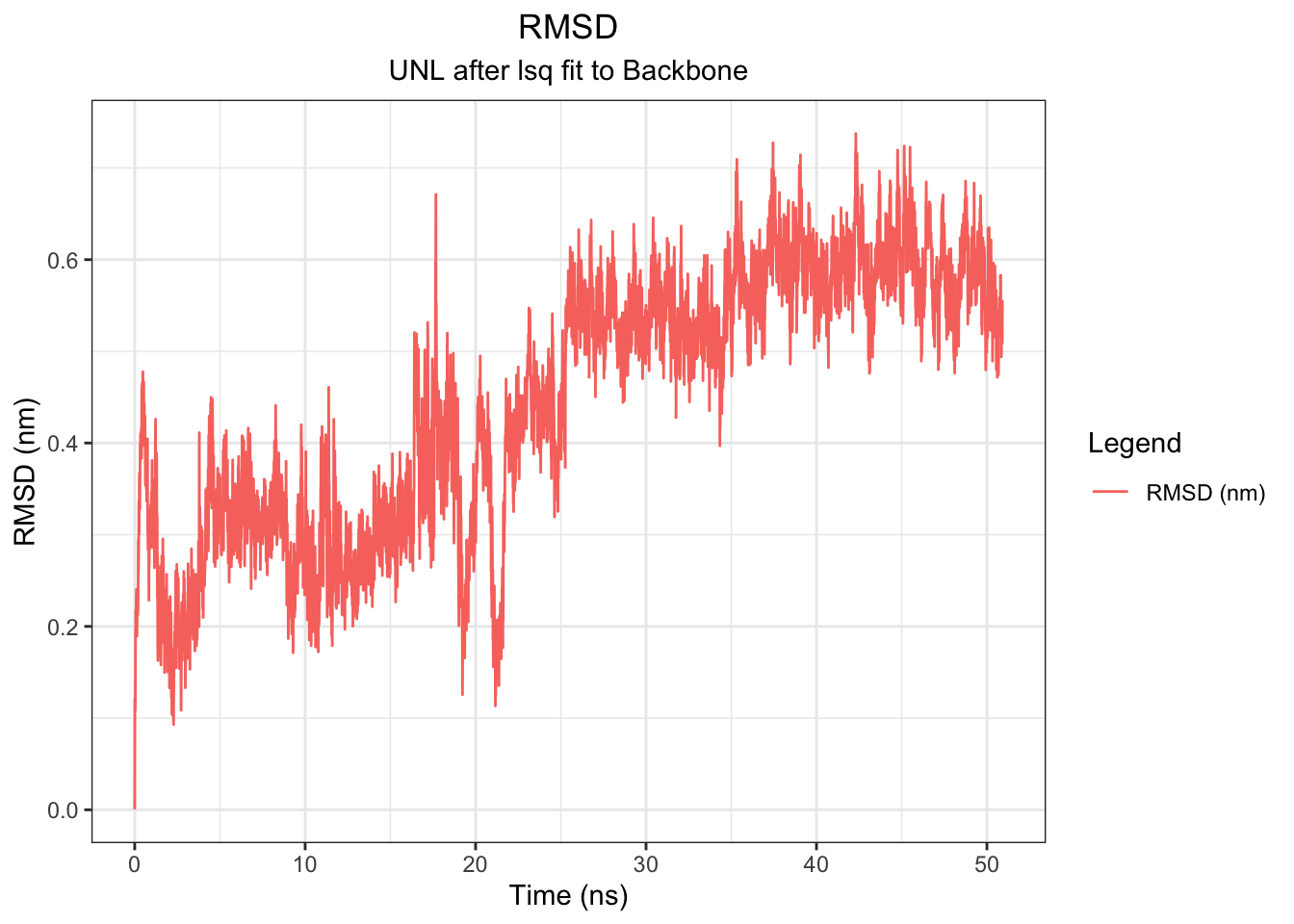
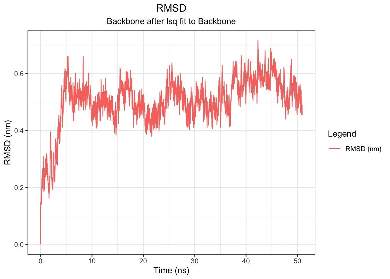
Backbone RMSD rises from 0 to ~0.5 nm within the first ~5 ns and plateaus around 0.5–0.6 nm for the remainder of the 50 ns simulation, indicating the protein equilibrates early and maintains a stable conformation throughout — consistent across all simulation lengths tested. The ligand (UNL) RMSD tells a different story: it fluctuates around 0.2–0.4 nm for the first ~20 ns, then drifts progressively upward to ~0.5–0.7 nm after ~25 ns with no plateau, suggesting the ligand undergoes a conformational transition away from its original docked pose mid-simulation. However, this should be interpreted alongside the minimum distance, COM distance, H-bond, and interaction energy data.

Note: I had to use echo “1 0” | gmx trjconv -s md.tpr -f md.xtc -o md_noPBC.xtc -pbc mol -center to re-center because there were some outliers of the RMSD of the ligand with 12-15 values. This disappeared after re-centering

Note: I also had to extend 10ns to 50ns to further assess if protein rmsd plateaud as it kept rising. To extend use this:

gmx convert-tpr -s md.tpr -extend 40000 -o md_extended.tpr

gmx mdrun -deffnm md_extended \
  -s md_extended.tpr \
  -cpi md.cpt \
  -nb gpu -pme gpu -bonded gpu -update gpu \
  -ntmpi 1 -ntomp 4 \
  -v

RMSF — Root Mean Square Fluctuation

What it measures: Per-residue (or per-atom) flexibility over time.

Identifies which regions of the protein and which atoms of the ligand are mobile. High flexibility at the binding site residues suggests the ligand isn’t holding them in place as expected.

# Per-residue protein flexibility
echo 4 | gmx rmsf -s md.tpr -f md_noPBC.xtc -o rmsf_protein.xvg -res 

# Per-atom ligand flexibility
echo 13 | gmx rmsf -s md.tpr -f md_noPBC.xtc -o rmsf_ligand.xvg 

Binding site residues with low RMSF (< 1–1.5 Å) = well-restrained by ligand. If RMSF of active site residues is HIGH while your ligand RMSD is also high → ligand is not stabilizing the pocket. What does our say?

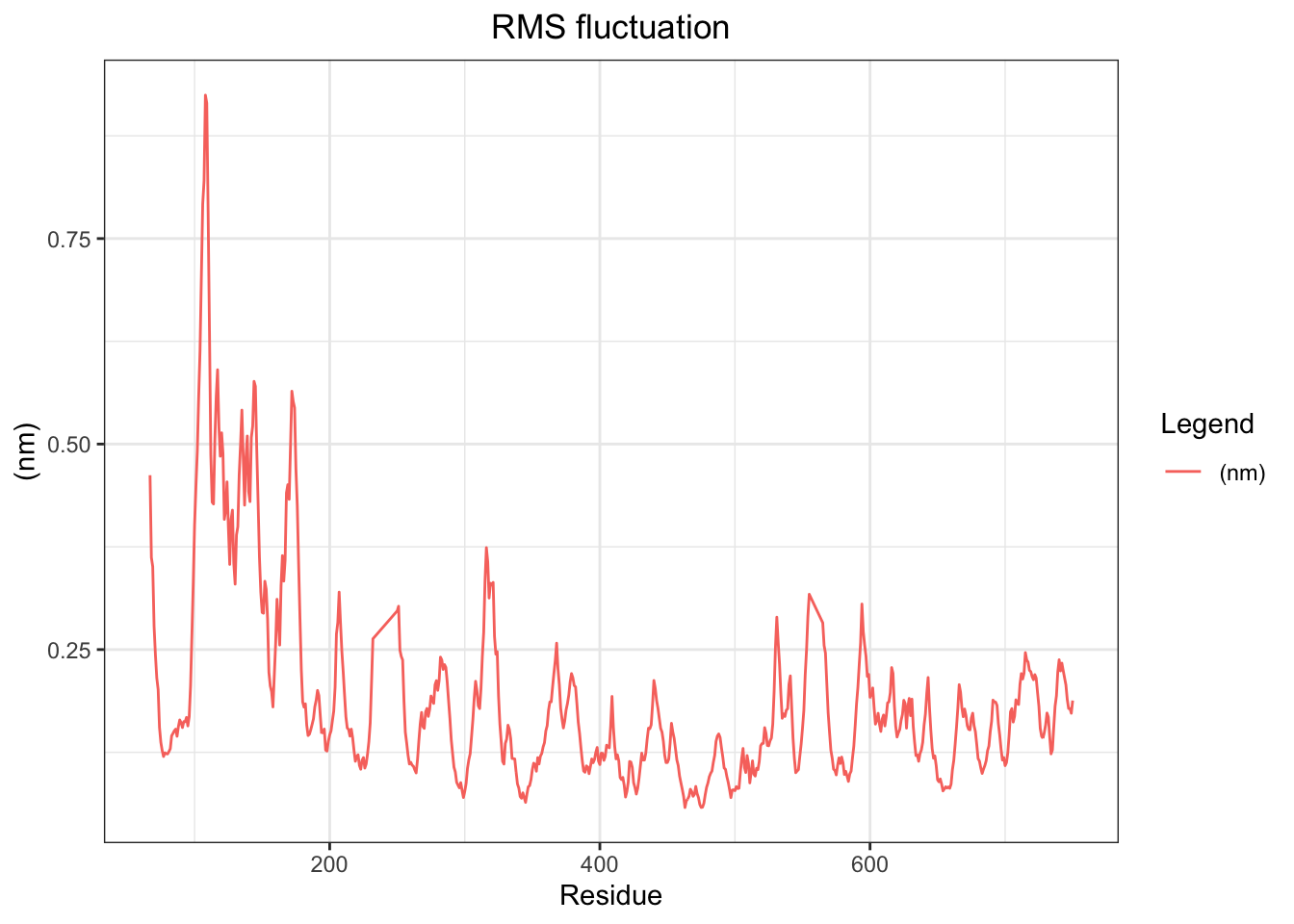
A few minor peaks around residues 200, 300, and 580–600 suggest localized loop flexibility mid-structure but nothing dramatic. Overall the RMSF profile is consistent with a stable, well-folded protein throughout the 50 ns simulation, with flexibility confined primarily to the N-terminal region as expected for a large multimeric protein like PBP2x.

rmsf_ligand <- read_xvg("rmsf_ligand.xvg")

plot_xvg(rmsf_ligand)

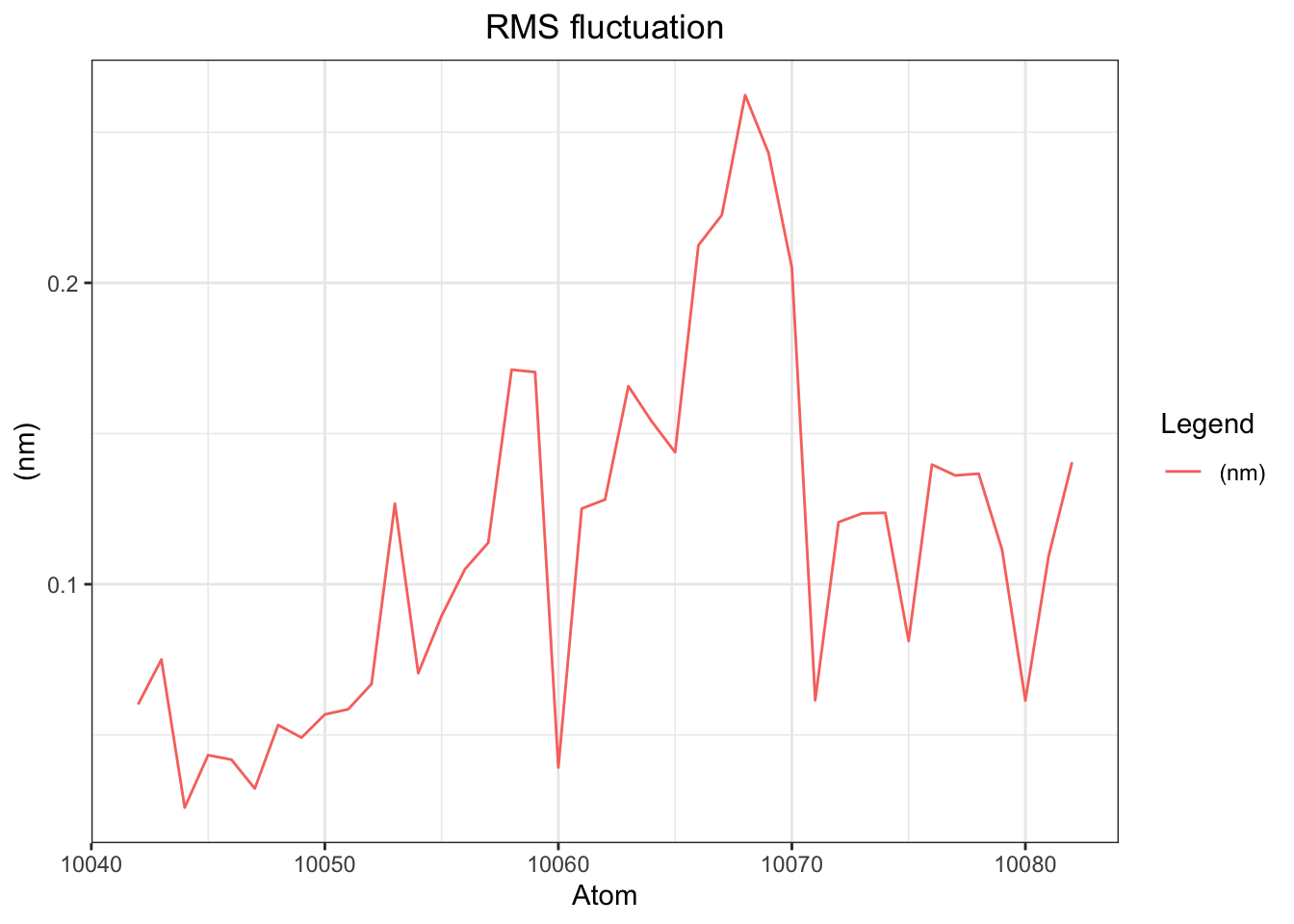
Ligand RMSF analysis shows per-atom fluctuations ranging from ~0.02–0.27 nm across all 41 atoms (system atoms 10041–10082), with a notable peak around atom 10068 corresponding to H7 on the aromatic ring region (benzene ring), suggesting this part of the ligand is the most dynamically flexible. Overall fluctuation levels are moderate and consistent with the dynamic pose sampling behavior observed throughout the simulation.

Now let’s visualize with ChimeraX and use color pallete of the temperature factor (bfactor) via gmx rmsf -s md.tpr -f md_noPBC.xtc -o rmsf.xvg -oq rmsf_bfactor.pdb -res. Blue means minimal wiggliness, white is middle, red is lots of wiggliness.

And we can see that (boxed by green color), our ligand rest quite comfortably in the pocket of prior cefepime with not a whole lot of wiggliness indicating not a whole lot of conformational change around the attached site.

Radius of Gyration (Rg)

What it measures: Compactness of the protein.

If the protein unfolds or the binding pocket opens/closes dramatically due to ligand binding/unbinding, Rg will change. It’s a global indicator of structural integrity.

echo '1' | gmx gyrate -s md.tpr -f md_noPBC.xtc -o gyrate.xvg 

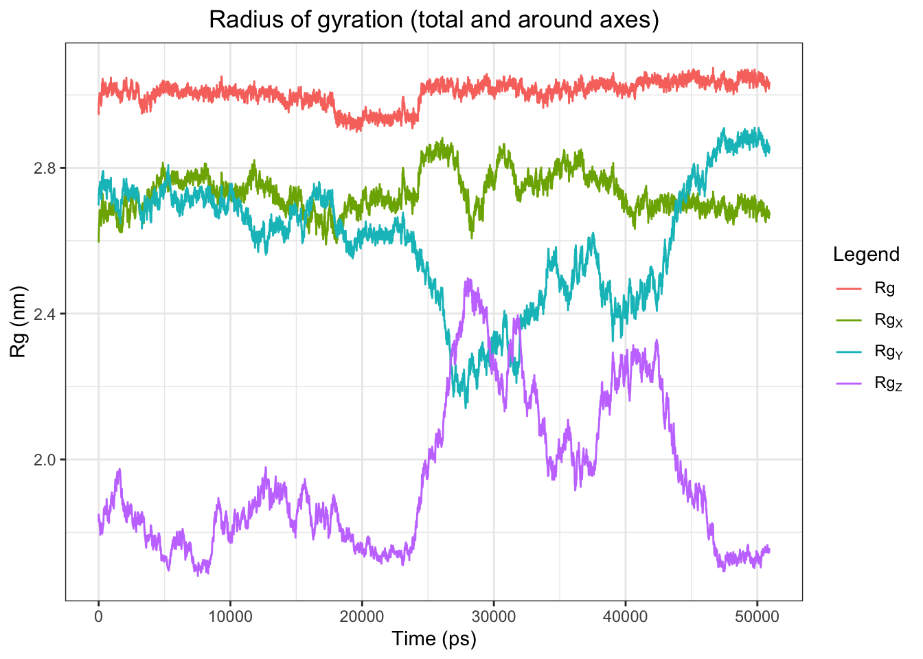
According to Claude, the radius of gyration plot for the 50 ns simulation shows total Rg remaining stable at ~2.9 nm throughout, confirming the protein maintains its overall fold with no unfolding or collapse. RgX stays relatively flat around ~2.75 nm. However RgY and RgZ show dramatic and unusual fluctuations between ~20,000–45,000 ps — RgY drops sharply from ~2.75 nm down to ~2.3 nm then recovers, while RgZ spikes from ~1.8 nm up to ~2.45 nm then returns to baseline. These large axial swings occurring simultaneously in opposite directions are concerning and could indicate significant domain reorganization, partial chain separation, or a PBC artifact requiring further investigation. Will visualize in ChimeraX to determine the cause.

In ChimeraX, load fullsystem.gro then load md_noPBC.xtc and enter command below. Then move to around 23000-30000 and see if it’s just a rotation.

hide solvent
hide :NA
hide :CL
cartoon
color bychain

Alright, it’s just a rotation! The RgY and RgZ fluctuations between ~20–45 ns are attributable to protein rotation/tumbling in the simulation box rather than genuine conformational change, as confirmed by visual inspection of the trajectory in ChimeraX. Total Rg remains flat throughout, and the axial variations reflect reorientation rather than structural instability. Overall the protein fold is well-maintained across the full 50 ns simulation

Ligand-Protein Interaction Energy

What it measures: Short-range Lennard-Jones (van der Waals) and Coulomb (electrostatic) energies between ligand and protein.

The most direct thermodynamic indicator. If the ligand is truly bound, the interaction energy should be negative (favorable) and stable. If it dissociates, the energy approaches 0.

Add this to md.mdp

energygrps = Protein UNL ; the UNL is your ligand, use whichever it's listed 

then rerun:

gmx grompp -f md.mdp -c md.gro -p topol.top -n index.ndx -o rerun.tpr
gmx mdrun -s rerun.tpr -rerun md_noPBC.xtc -e rerun.edr -ntmpi 1 -ntomp 4

gmx energy -f md.edr -o interaction_energy.xvg 

# then enter these
Coul-SR:Protein-LIG
LJ-SR:Protein-LIG
0

interaction <- read_xvg("interaction_energy.xvg")
plot_xvg(interaction)

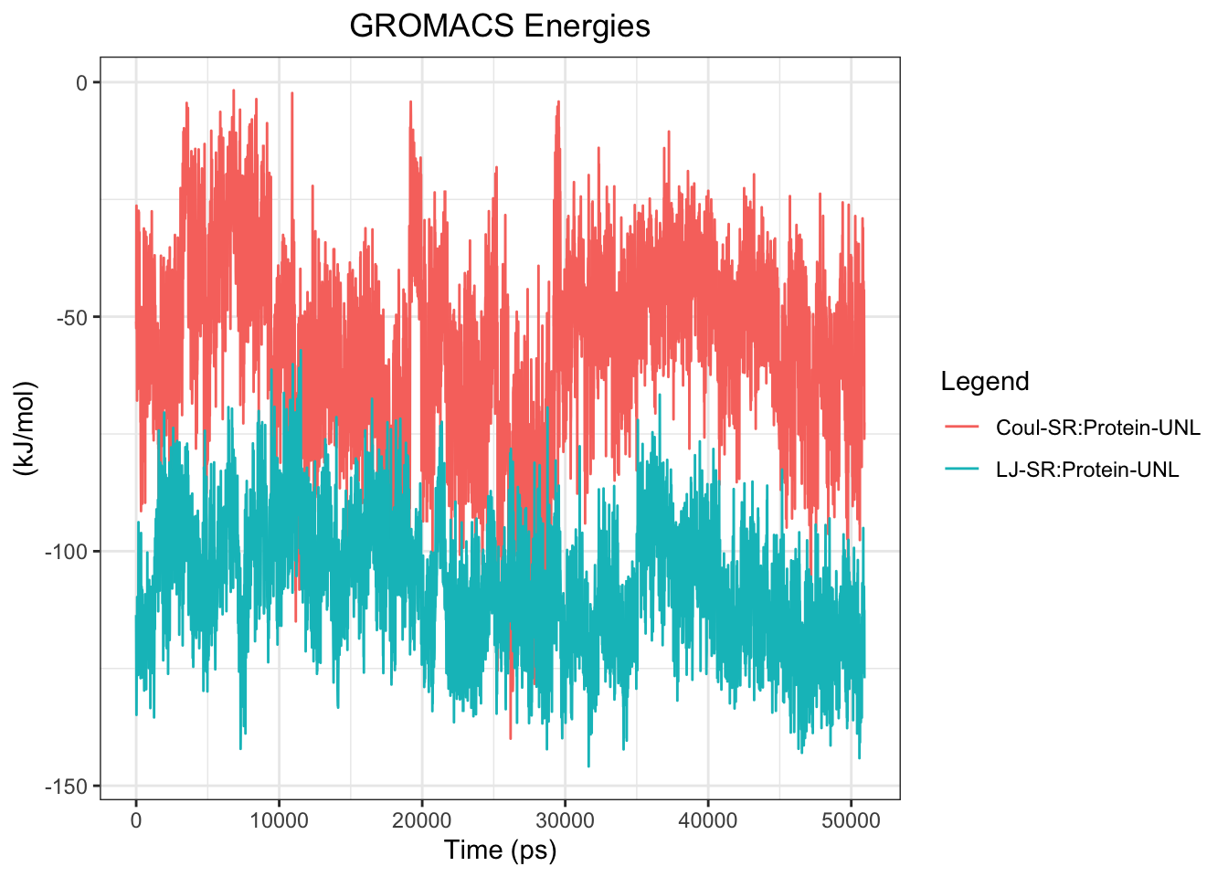
Interaction energy plots show LJ/vdW interaction is more stable and consistently negative (~-80 to -130 kJ/mol) throughout the simulation, while Coulomb interaction is highly variable (0 to -80 kJ/mol) with frequent excursions toward zero, indicating the ligand maintains physical contact with the protein but repeatedly loses and regains specific electrostatic interactions. This pattern is consistent with dynamic surface sampling rather than stable binding mode occupancy.

Note: For assessing interaction energy, we will have to rerun mdrun, only uses core, no gpu. But won’t take too long even for 50ns. I would do this after hbond. I tried to doing this together from the first production but it won’t let me.

Hydrogen Bond Analysis

What it measures: Number and occupancy of H-bonds between ligand and protein over the trajectory.

Critical for beta-lactam/PBP interactions — the acylation mechanism involves specific H-bonds. Persistent H-bonds = meaningful interaction.

more info than pdb during acpype conversion, so maybe try that out as well.

echo '1 13' | gmx hbond -s md.tpr -f md_noPBC.xtc -num hbond_ligand_protein.xvg -tu ns 

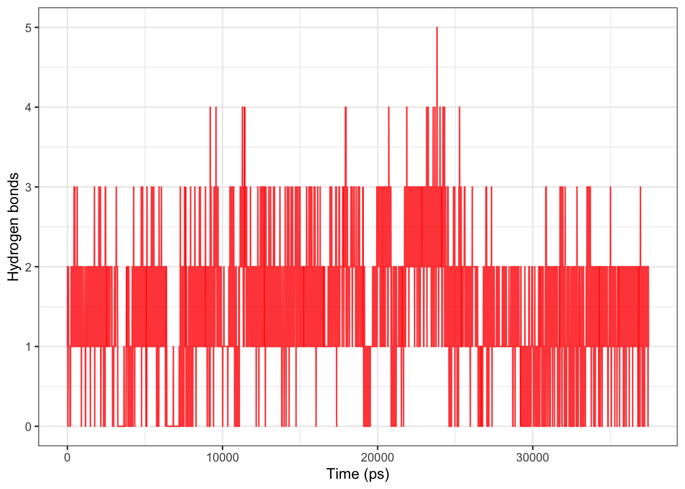
Ligand-protein H-bond analysis reveals 1–3 persistent H-bonds throughout the simulation with only rare drops to zero, indicating the ligand maintains contact with the protein but does not settle into a single stable binding pose — consistent with the progressive RMSD drift. Rather than full dissociation, the ligand appears to be dynamically sampling multiple interaction geometries. This suggests weak or non-specific binding at this site, and a more favorable docking pose or alternative binding site may need to be explored.

Note: Try simulating ligand-protein complex where you know it won’t bind and see this hydrogen bonds to be 0 0 0 0 all the way. Quite often, when i mistakenly docked in the wrong coordinates, my first few minutes production has very low hydrogen bond average. Usually in those situation, I’ll stop instead of continuing. What do you guys do?

Binding Pocket Distance Analysis

What it measures: Distance between the ligand center-of-mass (or key atoms) and key binding site residues.

RMSD can be misleading if the ligand rotates in place. Tracking distances to known catalytic residues (e.g., active site Ser, Lys, Thr in PBPs) gives mechanistically interpretable data.

# Distance between ligand COM and active site serine (e.g., residue 62, atom OG)
gmx distance -s md.tpr -f md_noPBC.xtc -oav distance_ser62.xvg -select 'com of group "LIG" plus atomname OG and resnum 62'

echo '1 13' | gmx mindist -f md_noPBC.xtc -s md.tpr -n index.ndx -od mindist_prot_lig.xvg -on numcont_prot_lig.xvg -d 0.4

gmx mindist -s md.tpr -f md_noPBC.xtc -od mindist_activesite.xvg -tu ns << EOF
13   # Ligand
r62  # Active site residue — create this group in make_ndx
EOF

gmx distance -f md_noPBC.xtc -s md.tpr -n index.ndx -select 'com of group "Protein" plus com of group "UNL"' -oall distance_prot_lig.xvg

mindist <- read_lines("mindist_prot_lig.xvg")

mindist_list <- mindist[!str_detect(mindist, "^@|^#")] |> str_split(" ")

time <- mindist_val <- vector(mode = "numeric", length = length(mindist_list))
for (i in 1:length(mindist_list)) {
  time[i] <- mindist_list[[i]][1]
  mindist_val[i] <- mindist_list[[i]][3]
}

mindist_df <- tibble(time = time, mindist_val = mindist_val) |>
  mutate(time = as.numeric(time),
         mindist_val = as.numeric(mindist_val))

plot_mindist <- mindist_df |>
  ggplot(aes(x=time,y=mindist_val)) +
  geom_point(color = "red", alpha=0.7) +
  theme_bw()

dist <- read_lines("distance_prot_lig.xvg")

dist_list <- dist[!str_detect(dist, "^@|^#")] |> str_trim() |> str_split("    ")

time <- dist_val <- vector(mode = "numeric", length = length(dist_list))
for (i in 1:length(dist_list)) {
  time[i] <- dist_list[[i]][1] 
  dist_val[i] <- dist_list[[i]][2]
}

dist_df <- tibble(time = time, dist_val = dist_val) |>
  mutate(time = as.numeric(time),
         dist_val = as.numeric(dist_val))

plot_dist <- dist_df |>
  ggplot(aes(x=time,y=dist_val)) +
  geom_point(color = "red", alpha=0.7) +
  theme_bw()

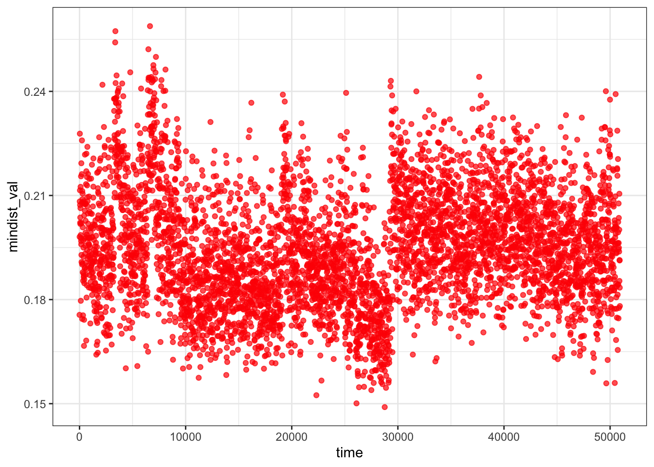
Minimum distance analysis between the ligand and protein confirms the ligand remains in close proximity (~0.15–0.25 nm) throughout the entire 50 ns simulation with no upward drift, ruling out full dissociation. Together with the persistent 1–3 protein-ligand H-bonds, this suggests the ligand maintains continuous contact with the protein surface but explores multiple binding geometries rather than converging on a single stable pose — consistent with weak or dynamic binding at this site.

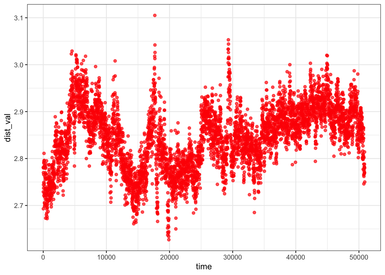
Center of mass distance between ligand and protein remains stable at ~2.75–2.95 nm throughout the 50 ns simulation with no directional drift, confirming the ligand does not dissociate from the protein. Combined with the minimum distance (~0.15–0.25 nm) and persistent 1–3 H-bonds, the collective picture is one of a ligand that remains associated with the protein but dynamically samples multiple surface poses rather than adopting a single locked binding mode — suggesting the binding interaction is real but relatively weak or non-specific at this site.

Visual Inspection

🙌 These trajectory is from the last few steps of the 50ns. looks like it’s still at the same place! Fantastic!

Let’s plot our frame 0 and frame 5000 and see where our ligand is.

# Extract full system at time 0
gmx trjconv -s md.tpr -f md_noPBC.xtc -o frame0.pdb -dump 0
# Select System

# Extract full system at time 50000
gmx trjconv -s md.tpr -f md_noPBC.xtc -o frame50000.pdb -dump 50000
# Select System

In ChimeraX, open both, then:

hide solvent
hide protein
hide :NA
hide :CL
cartoon
matchmaker #2 to #1 pairing bb
color #1:UNL red
color #2:UNL green
transparency 80 target c

The matchmaker aligns both frames.

Great! Looks like it the coordinates are quite similar! Especially the beta lactam ring area, which is the most important part for the interaction. The tail area seems to have more wiggle room, which is consistent with our RMSF analysis.

Wow, I learnt so much, and so much more to learn! The physics is really fascinating! I don’t understanding all of the them, but at least this is a step to knowing what I don’t know, which is a lot! The trials and erros we’ve gone through, and thanks to Claude, I was able to get unstuck! But still, took quite a long time from experimentation, reproducing with different pdbs, then the documentation! My heart goes to those who do this for a living… it’s not easy! ❤️ Thanks to all who contribute to the scientific community! All the software I used are freely available! And you can reproduce this at your own home as well! Please be sure to cite them!

Opportunities for Improvement

• Try out protein structures from AlphaFold Protein Structure Database
• Try out ColabFold
• Incorporate diffdock in discovering binding poses, compare it with fpocket, and perhaps also vina
• I was told that using mol2 directly has more info than pdb during acpype
• we did not assess covalent docking
• I need to turn all of the above into a pipeline where there is less copy and paste and typing! So I can run more!
• I am really curious about how certain ESBL beta lactamase has affinity to beta lactamase inhibitor. Want to see if gromacs can simulate this!
• I should really be using index in gromacs
• learn about MM-GBSA / MM-PBSA for post-processing

Lessons Learnt

• learn that you can use echo 15 | gmx something to insert 15 onto the next command response. Or gmx something << EOF 15 EOF
• learnt some basic gromacs workflow, interpretation, assessment
• learnt autodock vina and diffdock
• learnt to visualize with ChimeraX
• for GTX 1080, average around 40-50ns/day

If you like this article:

• please feel free to send me a comment or visit my other blogs
• please feel free to follow me on BlueSky, twitter, GitHub or Mastodon
• if you would like collaborate please feel free to contact me