From Math to Code: Building GAM with Penalty Functions From Scratch
By Ken Koon Wong in r R gam penalty gcv matrix calculus calculus derivative reimann sum taylor series
June 11, 2025
Enjoyed learning penalized GAM math. Built penalty matrices, optimized λ using GCV, and implement our own GAM function. Confusing? Yes! Rewarding? Oh yes!
We dove into the engine of what made basis spline work on our last blog, now let’s add to that and see how we can further improve the generalized additive model with penalty. Our previous linear regression model has a downside, it may overfit. Let’s see how we can minimize that with penalty function.
Objectives
- Equation of Linear Regression
- Add Penalty Parameter
- Proof of Derivate with Respect to Beta Coefficients
- Find Optimal Lambda
- Let’s Code
- Compare Our Custom Function vs mgcv::gam
- Applying this to Real Data
- Lessons Learnt
The End In Mind
Keep this at the back of our mind, our end goal is to understand this $$ \min (|| y - \beta x ||^2 + \lambda \beta^T S \beta) $$ Let’s split this up to two parts. The linear equation which is the left side, and the penalty equation which is the right.
Equation of Linear Regression
Let’s look the first equation, it’s basically ordinary least square.
$$ y = x \beta + \varepsilon \\ y - x \beta = \varepsilon $$
$$ \text{In order to ensure no negative values, we square the error} \\ (y - x \beta)^2 = \varepsilon^{2} $$
$$
\text{We then want to minimize the error squared} \\
\min \varepsilon^{2} = \min (y - x \beta)^2
$$
$$
\text{Sum over all error squared} \\
= \min \sum (y - x \beta)^2 \\
= (y - x \beta)^T (y - x \beta) \text{ which is the math trick for sum of squares}
$$
$$
\text{Expand the equation} \\
= y^T y - y^T (x \beta) - (x \beta)^T y + (x \beta)^T (x \beta) \\
= y^T y - 2 (x^T \beta)^T y + \beta^T (x^T x) \beta
$$
If you’re like me rusty in math, you might be wondering how did we get from the 2nd last equation to the last equation. Let’s break it down. Especially \(-2 (x^T \beta)^T y + \beta^T (x^T x) \beta\)
$$ -y^{T} (x \beta) - (x \beta)^{T} y \\ = -y^{T} (x \beta) - \beta^{T} x^{T} y \\ \text{because } s = s^{T} \text{ if scalar and both } y^{T} (x \beta) \text{ and } \beta^{T} x^{T} y \text{ are scalars} \\ \text{meaning} - \beta^{T} x^{T} y - \beta^{T} x^{T} y \\ = -2 (x^T \beta)^{T} y $$
Alright, as for the last term, we can see that \((x \beta)^T (x \beta)\) is the same as \(\beta^T (x^T x) \beta\) because of the property of transpose.
$$ (x \beta)^T (x \beta) \\ = \beta^T x^T x \beta $$ Matrix Derivates Cheat Sheet
Fantastic! Now let’s plug these into the original equation. $$ \min \sum (y - x \beta)^2 = \min (y^T y - 2 x^T \beta^T y + \beta^T x^T x \beta) $$
Add Penalty Parameter
Now we have the equation for linear regression, let’s add a penalty parameter \(\lambda\) to it. This is to prevent overfitting. The other part of the equation is the penalty term, which is \(\beta^T S \beta\) where \(S\) is a penalty matrix.
$$
\lambda \beta^T S \beta
$$
Where \(S\) is a penalty matrix, and \(\lambda\) is a penalty parameter.
How Do We Get Penalty Matrix (S)?
The penalty matrix \(S\) is typically derived from the second derivative of the basis functions. In the case of B-splines, it can be calculated as a difference matrix that captures the curvature of the spline. The second-order difference matrix is often used, which penalizes the second derivative of the spline function.
But how did we get to \(\beta^{T}S\beta\)? Now, beta \(\beta\) and \(B\) look similar, it was confusing for me to when we have all these equations. Let’s temporarily change \(\beta\) (Beta, aka coefficients we want to estiamte) to c as coefficients, and maintain \(B\) as the B-spline basis functions. 👍 So we have \(c^{T}Sc\), and S as penalty matrix.
OK. Let’s assume that this is some f(x) function where x is the grid point. And we essentially want to find the second derivative of the B-spline basis functions at these grid points. The second derivative is denoted as \(f''(x)\). We want to square it to be positive definite, so we have \(f''(x)^2\).
So, what f(x) are we trying to penalize here? You got it, the B-spline basis functions. We want to penalize the second derivative of the B-spline basis functions. Let’s refresh our memory on the B-spline basis functions. The B-spline basis functions are defined as follows:
$$ f(x) = c_1B_1(x) + c_2B_2(x) + … + c_nB_n(x) $$
Let’s just take 3 basis function just for exercise.
$$ f(x) = c_1B_1(x) + c_2B_2(x) + c_3B_3(x) $$
We want to square the second derivative of this function, so we have:
$$
f’’(x) = c_1B_1’’(x) + c_2B_2’’(x) + c_3B_3’’(x)
$$
Next, for positive definiteness, we square the second derivative:
$$
f’’(x)^2 = (c_1B_1’’(x) + c_2B_2’’(x) + c_3B_3’’(x))^2
$$
Now, we want to integrate this over the domain of the B-spline basis functions.
$$
\int f’’(x)^2 dx = \int (c_1B_1’’(x) + c_2B_2’’(x) + c_3B_3’’(x))^2 dx
$$
OK, now it becomes a tad scary. Let’s ignore the integration for now and try to expand the quadratic term:
$$
(c_1B_1’’(x) + c_2B_2’’(x) + c_3B_3’’(x))^2 \\
= c_1^2 B_1’’(x)^2 + c_2^2 B_2’’(x)^2 + c_3^2 B_3’’(x)^2 \\ + 2c_1c_2B_1’’(x)B_2’’(x) + 2c_1c_3B_1’’(x)B_3’’(x) + 2c_2c_3B_2’’(x)B_3’’(x) \\
\text{which eventually leads to} \\
= \sum_{i}^{n} \sum_{j}^{n} c_ic_j B_i’’(x)B_j’’(x) \\
$$
Still with me? Now let’s plug this back into our integration:
$$
\int f’’(x)^2 dx = \int \sum_{i}^{n} \sum_{j}^{n} c_ic_j B_i’’(x)B_j’’(x) dx \\
= \sum_{i}^{n} \sum_{j}^{n} c_ic_j \int B_i’’(x)B_j’’(x) dx
$$
We’ll come back to the \(c^{T}Sc\) proof. Now, let’s define the penalty matrix S as follows:
$$
S[i,j] = \int B_i’’(x)B_j’’(x) dx
$$
OK, how do we then calculate or estimate \(B_i''(x)\) ? We don’t have a formula or anything to get to the second derivative of the B-spline basis functions directly. Instead, we will use numerical integration to approximate the second derivative at the grid points. But how !?! In come, Taylor series approxiation, again!
The second derivative of a function at a point can be approximated using finite differences as follows using a general f(x):
$$
\text{foreward approximation} \\
f(x+h) \approx f(x) + f’(x)h + \frac{f’’(x)}{2}h^2 \\
\text{backward approximation} \\
f(x-h) \approx f(x) - f’(x)h + \frac{f’’(x)}{2}h^2
$$
Now, there is a mathematical trickery where we can use the forward and backward approximation to get to the second derivative by adding both together:
$$
\text{adding both together} \\
f(x+h) + f(x-h)
= (f(x) + f’(x)h + \frac{f’’(x)}{2}h^2) + (f(x) - f’(x)h + \frac{f’’(x)}{2}h^2) \\
f(x+h) + f(x-h) = 2f(x) + f’’(x)h^2 \\
f’’(x)h^2 = f(x+h) + f(x-h) - 2f(x) \\
f’’(x) = \frac{f(x+h) + f(x-h) - 2f(x)}{h^2}
$$
We basically just turn the f to B to go back to our S matrix (penalty matrix)
$$
B_i’’(x) = \frac{B_i(x+h) + B_i(x-h) - 2B_i(x)}{h^2}
$$
This is the same for \(B_j''\).
Now, we can plug this back into our penalty matrix S:
$$
S[i,j] = \int B_i’’(x)B_j’’(x) dx \\
= \int \frac{B_i(x+h) + B_i(x-h) - 2B_i(x)}{h^2} \cdot \frac{B_j(x+h) + B_j(x-h) - 2B_j(x)}{h^2} dx
$$
In this case we will use numerical integration to compute the penalty matrix. Meaning, we will use a grid of 100 evenly separated points to evaluate the B-spline basis functions and their second derivatives, and then compute the penalty matrix S. We have to ensure NOT to use the first and last point since we need to use both forward and backward approximation to get to the second derivative.
Example, let’s say we have 5 evenly separated points (this is very small, but just for illustration) and our min point is -5, max is 5, which means x = [-5, -2.5, 0, 2.5, 5] as our grid points. h here is our step size.
$$
h = \frac{5 - (-5)}{5 - 1} = \frac{10}{4} = 2.5
$$
Now let’s look at what \(B_i\) (pay attention, this is NOT the 2nd derivative) looks like with 3 basis function (columns), and 5 grid points (rows), these can be calculated from
cox deboor recursion, but you can just use spliness::bs(x=c(-5,-2.5,0,2.5,5)):
$$
\begin{bmatrix} 0 & 0 & 0 \\\ 0.42 & 0.14 & 0.02 \\\ 0.38 & 0.38 & 0.13 \\\ 0.14 & 0.42 & 0.42 \\\ 0 & 0 & 1 \end{bmatrix}
$$
Now we want to then use this formula \(\frac{B_i(x+h) + B_i(x-h) - 2B_i(x)}{h^2}\) to create \(B_i''(x)\) (the second derivative of the B-spline basis functions). Note that we don’t want to look at x=-5 and x=5.
Let’s look at \(B_1\) and \(x=-2.5\) as an example:
$$
B_1’’(x=-2.5) = \frac{B_1(x+2.5) + B_1(x-2.5) - 2B_1(x)}{2.5^2} \\
= \frac{B_1(x=0) + B_1(x=-5) - 2B_1(x=-2.5)}{2.5^2} \\
= \frac{0.38 + 0 - 2(0.42)}{2.5^2} \\
= \frac{0.38 - 0.84}{6.25}
$$
Alright, we don’t have to get the result, the above is just an example on how to use the formula. Now let’s construct our \(D\) matrix, which is a matrix of \(B_i''(x)\) with the above formula like so:
$$ D \\ = \begin{bmatrix} \frac{B_1(x_2+h) + B_1(x_2-h) - 2B_1(x_2)}{h^2} & \frac{B_2(x_2+h) + B_2(x_2-h) - 2B_2(x_2)}{h^2} & \frac{B_3(x_2+h) + B_3(x_2-h) - 2B_3(x_2)}{h^2} \\ \frac{B_1(x_3+h) + B_1(x_3-h) - 2B_1(x_3)}{h^2} & \frac{B_2(x_3+h) + B_2(x_3-h) - 2B_2(x_3)}{h^2} & \frac{B_3(x_3+h) + B_3(x_3-h) - 2B_3(x_3)}{h^2} \\ \frac{B_1(x_4+h) + B_1(x_4-h) - 2B_1(x_4)}{h^2} & \frac{B_2(x_4+h) + B_2(x_4-h) - 2B_2(x_4)}{h^2} & \frac{B_3(x_4+h) + B_3(x_4-h) - 2B_3(x_4)}{h^2} \end{bmatrix}` $$
Notie that we don’t have to calculate the first and last row since we don’t have the forward and backward approximation for those points.
Still with me? Let’s refresh on where we digressed. This \(S[i,j] = \int B_i''(x)B_j''(x) dx\) !!! How on earth do we integrate this? We don’t have to! We can use numerical integration to approximate the integral. In this case, we can use the trapezoidal rule or
Riemann’s sum to estimate.
$$
S[i,j] = \int B_i’’(x)B_j’’(x) dx \\
= \sum_{k=1}^{n} B_i’’(x_k)B_j’’(x_k) \cdot h \\
= D^{T} D \cdot h \\
\text{Because } \sum_{k=1}^{n} B_i’’(x_k)B_j’’(x_k) \text{ is essentially } D^{T} D
$$
Here is why \(\sum_{k=1}^{n} B_i''(x_k)B_j''(x_k)\) is essentially \(D^{T} D\):
$$
\sum_{k=1}^{n} B_i’’(x_k)B_j’’(x_k) \\
= \begin{bmatrix}
B_1’’(x_2) & B_1’’(x_3) & B_1’’(x_4) \\
B_2’’(x_2) & B_2’’(x_3) & B_2’’(x_4) \\
B_3’’(x_2) & B_3’’(x_3) & B_3’’(x_4)
\end{bmatrix} \cdot \begin{bmatrix}
B_1’’(x_2) & B_2’’(x_2) & B_3’’(x_2) \\
B_1’’(x_3) & B_2’’(x_3) & B_3’’(x_3) \\
B_1’’(x_4) & B_2’’(x_4) & B_3’’(x_4)
\end{bmatrix} \\
= D^{T} D
$$
This \(D^{T} D \cdot h\) is ultimately our \(S\) matrix, which is the penalty matrix.
OK, now let’s bring this equation back to our original equation: $$ \int f’’(x)^2 dx = \int \sum_{i}^{n} \sum_{j}^{n} c_ic_j B_i’’(x)B_j’’(x) dx \\ = \sum_{i}^{n} \sum_{j}^{n} c_ic_j \int B_i’’(x)B_j’’(x) dx \\ = \sum_{i}^{n} \sum_{j}^{n} c_ic_j S[i,j] \\ = c^{T} S c $$
Now you may ask how on earth did we go from \(\sum_{i}^{n} \sum_{j}^{n} c_ic_j S[i,j]\) to \(c^{T} S c\)
Let’s set an example:
$$
c = \begin{bmatrix}
c_1 \\
c_2 \\
c_3
\end{bmatrix} ,
S = \begin{bmatrix}
S_{1,1} & S_{1,2} & S_{1,3} \\
S_{2,1} & S_{2,2} & S_{2,3} \\
S_{3,1} & S_{3,2} & S_{3,3}
\end{bmatrix}
$$
Now we know that \(\sum\) in coding is basically a for loop, hence \(\sum_{i}^{n} \sum_{j}^{n} c_ic_j S[i,j]\) means we have a nested for loop on another for loop. If we were to expand this it will look like
$$
\sum_{i}^{n} \sum_{j}^{n} c_ic_j S[i,j] \\
= c_1c_1S_{1,1} + c_1c_2S_{1,2} + c_1c_3S_{1,3} + \\
c_2c_1S_{2,1} + c_2c_2S_{2,2} + c_2c_3S_{2,3} + \\
c_3c_1S_{3,1} + c_3c_2S_{3,2} + c_3c_3S_{3,3}
$$
How we then turn these into \(c^{T}Sc\) is the following magic matrix operation.
- Rearrange
$$ c_1(S_{1,1}c_1 + S_{1,2}c_2 + S_{1,3}c_3) + \\ c_2(S_{2,1}c_1 + S_{2,2}c_2 + S_{2,3}c_3) + \\ c_3(S_{3,1}c_1 + S_{3,2}c_2 + S_{3,3}c_3) $$
- Notice how we can use matrix multiplication to express this as a dot product:
$$ `\begin{bmatrix} S_{1,1}c_1 + S_{1,2}c_2 + S_{1,3}c_3 \\ S_{2,1}c_1 + S_{2,2}c_2 + S_{2,3}c_3 \\ S_{3,1}c_1 + S_{3,2}c_2 + S_{3,3}c_3 \end{bmatrix} = \begin{bmatrix} S_{1,1} & S_{1,2} & S_{1,3} \\ S_{2,1} & S_{2,2} & S_{2,3} \\ S_{3,1} & S_{3,2} & S_{3,3} \end{bmatrix} \cdot \begin{bmatrix} c_1 \\ c_2 \\ c_3 \end{bmatrix} \\ = S \cdot c \\ \text{In order to get to } c^{T}Sc \text{ we need to transpose } c \text{, hence} \\ c^{T}Sc = \begin{bmatrix} c_1 & c_2 & c_3 \end{bmatrix} \cdot \begin{bmatrix} S_{1,1} & S_{1,2} & S_{1,3} \\ S_{2,1} & S_{2,2} & S_{2,3} \\ S_{3,1} & S_{3,2} & S_{3,3} \end{bmatrix} \cdot \begin{bmatrix} c_1 \\ c_2 \\ c_3 \end{bmatrix} \\ = c_1(S_{1,1}c_1 + S_{1,2}c_2 + S_{1,3}c_3) + \\ c_2(S_{2,1}c_1 + S_{2,2}c_2 + S_{2,3}c_3) + \\ c_3(S_{3,1}c_1 + S_{3,2}c_2 + S_{3,3}c_3) \\ \text{which is essentially a scalar!} $$
Phew, all those math gymnastics and acrobatics! Worked out a sweat, don’t they? Now, remember we switch \(\beta\) to c, these are coefficients, so that we don’t confuse \(\beta\) (beta) with B, our basis function? OK, now that basis function is long “gone”, we will then turn \(c^{T}Sc\) back to \(\beta^{T}S\beta\) for consistency with general notation.
And there you have it! We have derived the penalty term \(\beta^{T}S\beta\) in the generalized additive model with B-spline basis functions.
Proof of Derivate with Respect to Beta Coefficients
Now that we have the penalty term, let’s take the derivative of the entire equation with respect to \(\beta\):
$$ \min (|| y - \beta x ||^2 + \lambda \beta^T S \beta) \\ = \min (y^T y - 2 x^T \beta^T y + \beta^T x^T x \beta + \lambda \beta^T S \beta) $$
Taking the derivative with respect to \(\beta\) gives us:
$$
\frac{\partial}{\partial \beta} (y^T y - 2 x^T \beta^T y + \beta^T x^T x \beta + \lambda \beta^T S \beta) \\
= 0 -2 x^T y + 2 x^T x \beta + 2 \lambda S \beta
$$
Setting the derivative to zero gives us the normal equations:
$$
0 - 2 x^T y + 2 x^T x \beta + 2 \lambda S \beta \\
2 x^T y = 2 x^T x \beta + 2 \lambda S \beta \\
x^T y = x^T x \beta + \lambda S \beta \\
\beta (x^T x + \lambda S) = x^T y \\
\beta = (x^T x + \lambda S)^{-1} x^T y
$$
OK. We went through ALL those trouble to find out the equation to find beta coefficients for After all these, what on earth is lambda !?!?!
What is Lambda
Lambda is a penalty parameter that controls the amount of regularization applied to the model. It is a hyperparameter that you can tune to find the optimal balance between fitting the data and preventing overfitting. A larger lambda value will result in more regularization, while a smaller value will result in less regularization. lambda = 0 means no penalty, it is equivalent to ordinary least squares regression. Once we found the optimal lambda, we can plug that number in to calculate our beta, how cool! Now how to we find the optimal lambda?
Generalized Cross Validated (GCV)
To find the optimal lambda, we can use Generalized Cross Validation (GCV). GCV is a method that estimates the prediction error of a model by minimizing the GCV score. The GCV score is defined as follows:
$$ \text{GCV} = \frac{n \times RSS}{(n - \text{trace}(H))^2} $$
Where \(\hat{y}\) is the predicted value, and \(H\) is the hat matrix. The trace of the hat matrix is the sum of the diagonal elements of the hat matrix, which is the number of parameters in the model. The GCV score is a measure of how well the model fits the data, and we want to minimize this score to find the optimal lambda.
Find Optimal Lambda
In other words:
Step 1. Calculate H (hat matrix)
$$ H = X(X^T X + \lambda S)^{-1} X^T $$
Step 2. Calculate \(\hat{y}\) (predicted value)
$$ \hat{y} = H y $$
Step 3. Calculate RSS
$$ RSS = || y - \hat{y} ||^2 $$ Step 4. Calculate GCV score
$$
\text{GCV}(\lambda) = \frac{n \times RSS}{(n - \text{trace}(H))^2}
$$
Step 5. Find the optimal lambda that minimizes the GCV score. Et viola!
Let’s Code
Now, we did A LOT of math there, let’s bring down the essential formulae as a reminder. But first, let’s simulate some non-linear data!
library(tidyverse)
library(splines)
library(mgcv)

set.seed(123)
n <- 1000
z <- runif(n,-5,5)
y <- sin(z) + rnorm(n,0.1)
df <- tibble(z = z, y = y)

df |>
  ggplot(aes(x = z, y = y)) +
  geom_point(alpha=0.5)

This should be pretty straight forward. We’ve seen this before in our previous blog.
Penalty Matrix
$$ S[i,j] = \int B_i’’(x)B_j’’(x) dx \\ = \sum_{k=1}^{n} B_i’’(x_k)B_j’’(x_k) \cdot h \\ = D^{T} D \cdot h \\ \text{Because } \sum_{k=1}^{n} B_i’’(x_k)B_j’’(x_k) \text{ is essentially } D^{T} D $$
penalty_matrix <- function(z_vals, n_basis, n_grid = 100) {
  # Step 1: Create fine grid over the domain
  z_min <- min(z_vals)
  z_max <- max(z_vals)
  z_grid <- seq(z_min, z_max, length.out = n_grid)
  h <- z_grid[2] - z_grid[1]

  # Step 2: Evaluate B-spline basis functions on the grid
  X_grid <- bs(z_grid, df = n_basis, intercept = TRUE)

  # Step 3: Compute second derivatives using finite differences; Also known as Bi" or Bj" here (Basis, not beta), or D
  D <- matrix(0, n_grid - 2, n_basis)

  for (i in 2:(n_grid - 1)) {
    for (j in 1:n_basis) {
      D[i-1, j] <- (X_grid[i-1, j] - 2*X_grid[i, j] + X_grid[i+1, j]) / h^2
    }
  }

  # Step 4: Compute penalty matrix S[i,j] = ∫ B''ᵢ(x) B''ⱼ(x) dx
  S <- t(D) %*% D * h

  return(S)
}
The above is our penalty matrix, basically to calculate S.
Find the Minimum GCV
$$ \text{GCV}(\lambda) = \frac{n \times RSS}{(n - \text{trace}(H))^2} $$
# y <- df_bs$n
# z <- seq(1,length(df_bs$date),1)
n_basis <- 10
x <- bs(z, df = n_basis, intercept=T)
# s <- penalty_matrix(n_basis)
s <- penalty_matrix(z,n_basis=n_basis)
lambda_vec <- seq(0,10,0.01)


gcv <- numeric(length(lambda_vec))
# GCV function
for (i in 1:length(lambda_vec)) {
  lambda <- lambda_vec[i]

  # 1. Calculate H = x(xᵀx + λS)⁻¹xᵀ
  H <- function(lambda, x, s) {
    # Calculate H
    H <- x %*% solve(t(x) %*% x + lambda * s) %*% t(x)
    return(H)
  }

  h <- H(lambda,x, s)

  # 2. Calculate ŷ = Hy
  y_hat <- h %*% y

  # 3. Calculate RSS = ||y - ŷ||²
  rss <- sum((y-y_hat)^2)

  # 4. Calculate GCV(λ) = (n × RSS) / (n - tr(H))²
  tr_H <- sum(diag(h))
  gcv_value <- (n * rss) / ((n - tr_H)^2)

  gcv[i] <- gcv_value
}

tibble(lambda=lambda_vec, gcv=gcv) |>
  ggplot(aes(x=lambda, y=gcv)) +
  geom_line() +
  labs(title="GCV vs Lambda", x="Lambda", y="GCV") +
  theme_minimal()
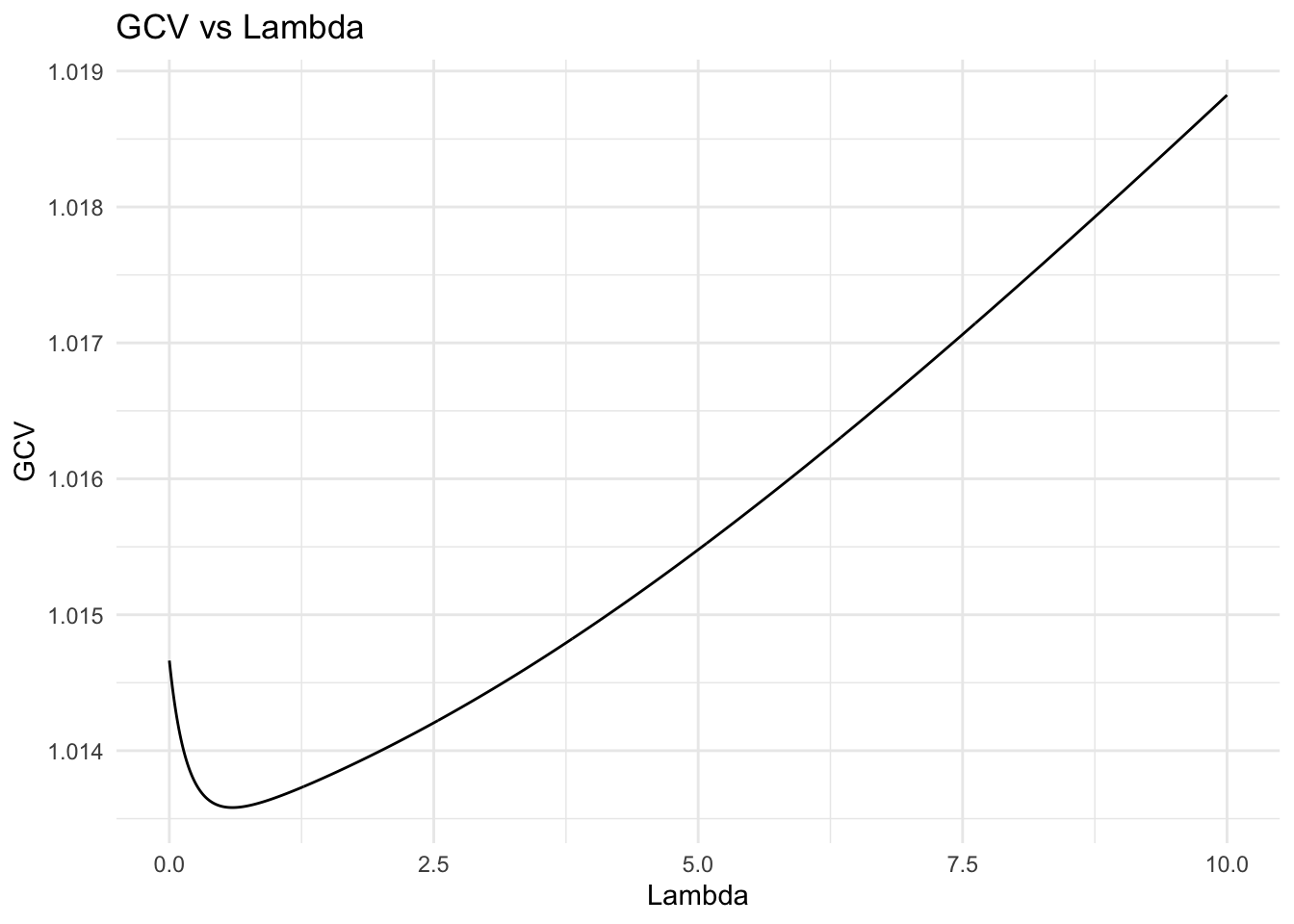
## optimal lambda
(opt_lambda <- lambda_vec[which(gcv==min(gcv))])
## [1] 0.6
(min_gcv <- min(gcv_value))
## [1] 1.018823
Alright, the plot shows GCV value vs lambda. We essentially want to find lambda with the lowest GCV value. opt_lambda is the optimal lambda value. We then use this number to calculate our beta coefficients
Find Beta Coefficients
$$ \beta = (x^T x + \lambda S)^{-1} x^T y \\ $$
(beta <- solve(t(x) %*% x + opt_lambda * s) %*% t(x) %*% y)
##          [,1]
## 1   1.2375133
## 2   1.1800055
## 3   0.8037137
## 4  -1.2787422
## 5  -0.6854527
## 6   1.0479672
## 7   1.3246798
## 8  -0.4118710
## 9  -1.2195539
## 10 -0.8501258
Compare Our Custom Function vs mgcv::gam
# using mgcv::gam
model_gam <- gam(y~s(z, k=n_basis, bs = "bs"))

# turn our calculated beta to vector
beta <- as.vector(beta)

# Plotting the results
tibble(z, y) |>
  ggplot(aes(z, y)) +
  geom_point(alpha=0.2) +
  geom_line(aes(x = z, y = x %*% beta), color = "blue", size=2, alpha=0.5) +
  geom_line(aes(x = z, y = predict(model_gam)), color = "red", size = 2, alpha=0.5) +
  labs(x = "z", y = "y") +
  ggtitle(label = "GAM Fit with Custom Penalty Matrix and mgcv Package") +
  theme_minimal()

Wow, look at that! The blue line is our custom function, and the red line is the mgcv::gam function. They look pretty similar, right? As you can see we have blue for our custom gam and red as mgcv::gam. We get a purple color!
Let’s Try A Real Dataset, Our Very Own #IDsky
Now let’s try a different dataset, let’s look at Bluesky #IDsky posts counts
# Load the dataset
load("df_bs.rda")

# Some data wrangling
y <- df_bs$n
z <- seq(1,length(df_bs$date),1)

# Create B-spline basis functions
n_basis <- 20
x <- bs(z, df = n_basis, intercept=T)
s <- penalty_matrix(z,n_basis=n_basis,n_grid = 200)

# find optimal lambda
lambda_vec <- seq(44,48,0.001)

gcv <- numeric(length(lambda_vec))

# GCV function
for (i in 1:length(lambda_vec)) {
  lambda <- lambda_vec[i]

  # 1. Calculate H = x(xᵀx + λS)⁻¹xᵀ
  H <- function(lambda, x, s) {
    # Calculate H
    H <- x %*% solve(t(x) %*% x + lambda * s) %*% t(x)
    return(H)
  }

  h <- H(lambda,x, s)

  # 2. Calculate ŷ = Hy
  y_hat <- h %*% y

  # 3. Calculate RSS = ||y - ŷ||²
  rss <- sum((y-y_hat)^2)

  # 4. Calculate GCV(λ) = (n × RSS) / (n - tr(H))²
  tr_H <- sum(diag(h))
  gcv_value <- (n * rss) / ((n - tr_H)^2)

  gcv[i] <- gcv_value
}

tibble(lambda=lambda_vec, gcv=gcv) |>
  ggplot(aes(x=lambda, y=gcv)) +
  geom_line() +
  labs(title="GCV vs Lambda", x="Lambda", y="GCV") +
  theme_minimal()

## optimal lambda
(opt_lambda <- lambda_vec[which(gcv==min(gcv))])
## [1] 45.505
(min_gcv <- min(gcv_value))
## [1] 129.3409
(beta <- solve(t(x) %*% x + opt_lambda * s) %*% t(x) %*% y)
##          [,1]
## 1    3.444439
## 2    6.746956
## 3   -3.840163
## 4   15.139798
## 5   -5.688893
## 6   32.633905
## 7  -31.848643
## 8   75.342451
## 9  192.032407
## 10  44.874593
## 11  48.429720
## 12  65.626734
## 13  54.892071
## 14  86.819061
## 15  53.498207
## 16  55.391699
## 17  67.752137
## 18  21.012682
## 19  77.276639
## 20  33.333471
# compare mgcv::gam
model_gam <- gam(y~s(z, k=n_basis, bs = "bs"))
beta <- as.vector(beta)

# visualize
tibble(z, y) |>
  ggplot(aes(z, y)) +
  geom_point(alpha=0.2) +
  geom_line(aes(x = z, y = x %*% beta), color = "blue", size=2, alpha=0.5) +
  geom_line(aes(x = z, y = predict(model_gam)), color = "red", size = 2, alpha=0.5) +
  labs(x = "z", y = "y") +
  ggtitle(label = "GAM Fit with Custom Penalty Matrix and mgcv Package") +
  theme_minimal()
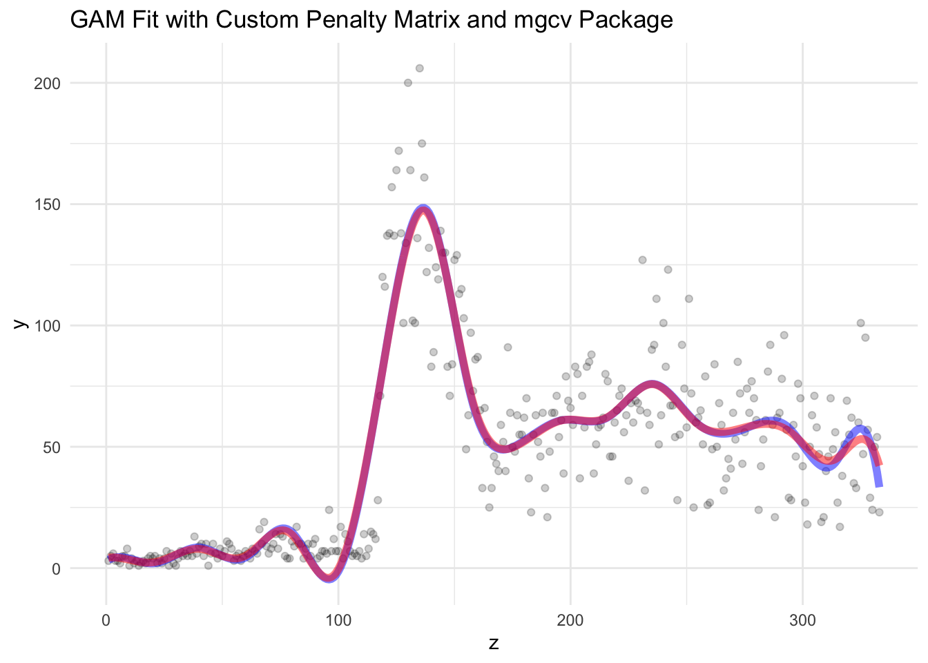
Look at that ! They are quite similar, aren’t they? Yes, we did it!!! PHew, that was a lot of math and coding!
Opportunities for Improvement
- Need to learn how to do the same for REML
Lessons Learnt
- learnt lots of lots of math behind GAM with penalty
- learnt how to derive the penalty matrix
- refresh on matrix operations, calculus, and algebra
If you like this article:
- please feel free to send me a comment or visit my other blogs
- please feel free to follow me on BlueSky, twitter, GitHub or Mastodon
- if you would like collaborate please feel free to contact me
- Posted on:
- June 11, 2025
- Length:
- 18 minute read, 3737 words
- Categories:
- r R gam penalty gcv matrix calculus calculus derivative reimann sum taylor series